

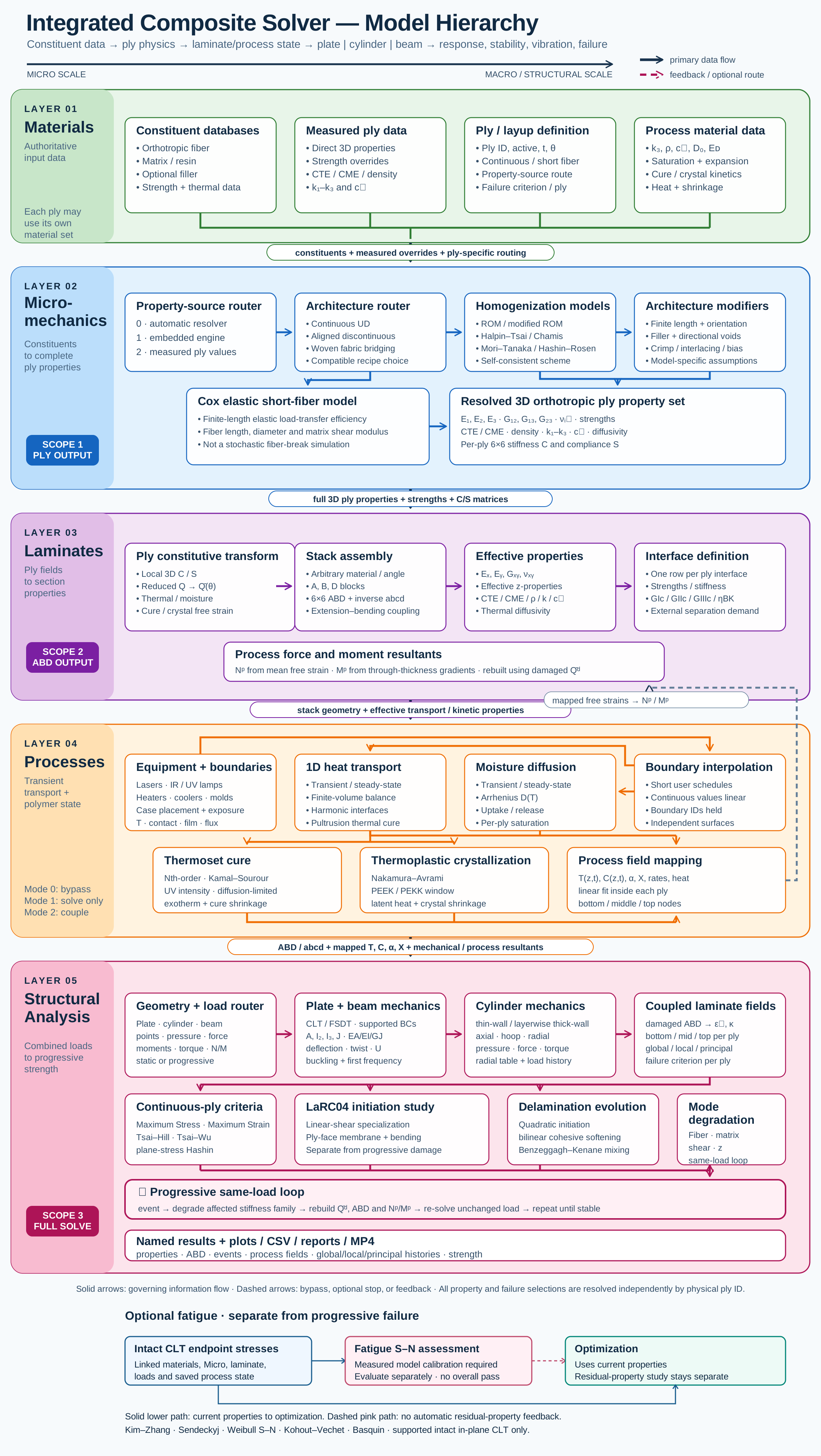
 Open the interactive Model Map
How to read this manual
Follow the workflow from physical assumptions and material data to ply and laminate properties, transport, structural response and design assessment. The chapters explain what is solved, what information crosses each connection and where the idealization stops. Detailed derivations remain linked within each chapter. Operating instructions belong in the User Guide; worked studies belong in the Training Manual.
This edition describes the established theory and currently documented solver boundaries. Model additions still being developed are not presented as released capabilities. Existing downloadable editions retain their stated release dates until their native Word and PDF replacements have been regenerated and reviewed.
Chapter 1
Model hierarchy and solver foundations
A CDS study is a dependency graph, not an isolated equation. Material records, constitutive models, ply definitions, geometry and boundary conditions determine which equations can be solved. Results belong to the input state used for that run; changing a linked record does not update an earlier stored solution.
1.1 Physical model and numerical model
Choose the physical idealization before choosing numerical resolution. A through-thickness transport model assumes in-plane uniformity. A laminate membrane model does not resolve local contact or a three-dimensional edge field. More nodes or smaller steps improve the numerical approximation within an idealization; they do not remove that idealization's limits.
1.2 Units and coordinate systems
Constituent and ply properties use material axes, while loading and geometry use structural axes. State the transformation convention, engineering shear convention, thickness direction and stress signs. Convert units at interfaces rather than mixing unit systems inside a stiffness or transport operator.
1.3 Execution sequence
Resolve linked records and model compatibility, assemble material and laminate properties, apply initial and boundary conditions, advance the selected fields, recover stresses and evaluate failure measures. An unsupported coupling must remain explicitly excluded. A successful run is a numerical outcome, not evidence of design qualification.
Detailed formulations
Back to contentsChapter 2
Material data and constitutive state
Every downstream prediction depends on the material definition. Separate measured values, fitted model coefficients, estimated properties and illustrative defaults. Record temperature, moisture condition, processing state, units and source with the values rather than treating a material name as a complete specification.
2.1 Elasticity and transport data
Elastic moduli, Poisson ratios and shear moduli define the stiffness response. Density, heat capacity, conductivity, moisture diffusivity and equilibrium uptake define different physical properties and cannot be inferred from stiffness alone. Orthotropic data must respect reciprocal compliance relationships and a physically admissible stiffness matrix.
2.2 State dependent properties
Cure and crystallization are internal state variables. Their kinetics, heat release and shrinkage require independent parameter definitions and calibration. A strength allowable does not automatically evolve because the elastic modulus or degree of cure changes. Use only the state dependencies implemented by the selected constitutive branch.
2.3 Data provenance
Document the applicable property range and interpolation policy. Extrapolation beyond measured temperatures, moisture levels or strain rates is a separate modeling assumption. Illustrative teaching records should remain labeled throughout the result and report.
Detailed formulations
References: [1]
Back to contentsChapter 3
Constituents to effective ply properties
Micromechanics maps constituent properties and architecture to an effective ply. The calculation requires a representative reinforcement arrangement and volume fractions. It does not replace measured design allowables or establish that a manufactured material has the assumed architecture.
3.1 Homogenization assumptions
Mixture estimates, inclusion models and shear-lag models make different assumptions about load transfer, geometry and interaction. Continuous aligned fibers, short fibers, fabrics and particle-filled systems require different architecture descriptions. Verify constituent limits and the effect of orientation and aspect ratio before comparing a predicted effective modulus with a test.
3.2 Property transfer
Pass the effective elastic tensor, density and directional expansion and transport properties with their coordinate convention. Retain separate provenance for each property family. A model calibrated for elastic stiffness is not automatically calibrated for thermal conductivity, diffusion or strength.
Detailed formulations
References: [1]
Back to contentsChapter 4
Ply transformations and laminate constitutive response
A laminate combines independently defined plies through their thicknesses, orientations and constitutive properties. Classical laminate theory represents in-plane strain as a mid-plane strain plus a term linear in the thickness coordinate. Integrating transformed ply stiffness produces the membrane, coupling and bending blocks.
4.1 Stiffness assembly
The A block relates membrane strain to membrane force, B represents extension–bending coupling and D relates curvature to bending moment. Symmetry of a correctly assembled layup eliminates B to numerical precision; balance alone does not guarantee symmetry. The stacking order and ply thickness must remain explicit.
4.2 Free strains and stress recovery
Thermal expansion, moisture expansion and any enabled process shrinkage are free strains. Integrate their equivalent force and moment resultants with the same ply definitions used for stiffness. Recover elastic strain by subtracting free strain before calculating stress. A free laminate can curve while its net force and moment remain zero; zero applied load does not imply zero ply stress.
Equation details — explanation, variables and reference
Applied force and moment equal the constitutive response minus the enabled free-strain resultants. Move the free-strain vector to the load side when solving for strain and curvature.
N: membrane force per width (N/m); M: moment per width (N); A, B, D: stiffness blocks (N/m, N, N·m); ε⁰: mid-plane strain; κ: curvature (1/m); starred resultants: integrated free-strain contributions.
Theory basisDetailed formulations
References: [1]
Back to contentsChapter 5
Heat transport and polymer evolution
Processing predicts the material history rather than simply prescribing the oven or die temperature to every ply. Heat conduction, boundary transfer and internal heat generation jointly determine the temperature field. Cure or crystallization can feed heat back into that field when the selected coupled model supports the reaction source.
5.1 Initial and surface conditions
Initial temperature is a material state. Surface schedules describe prescribed temperature, film transfer, insulation or flux; these are not interchangeable. Independent upper and lower boundaries can generate asymmetric fields. A finite film coefficient permits the material surface to lag the surrounding environment.
5.2 Coupling and time integration
Evaluate the kinetic rate using the local temperature and state, update reaction heat consistently with the mass basis of the enthalpy, and advance the thermal balance. A temperature rise attributable to reaction should be distinguished from the total material temperature. Check temporal and spatial refinement and compare integrated heat storage, boundary flux and internal generation.
5.3 Moving process coordinates
A constant-speed pultrusion model may map residence time to position using the pulling speed. This moving-section description does not by itself include axial conduction, resin flow, die deformation or pulling forces. UV and crystallization branches require their own calibrated input laws; they are not merely alternate thermal schedules.
Equation details — explanation, variables and reference
For the stationary one-dimensional conduction idealization, local heat storage balances conductive transfer and the enabled volumetric source. This is a conservation equation, not a complete cure law.
ρ: density (kg/m³); cp: specific heat (J/kg/K); T: temperature; t: time (s); z: thickness coordinate (m); kz: conductivity (W/m/K); q̇: volumetric heat generation (W/m³).
Theory basisDetailed formulations
References: [5]
Back to contentsChapter 6
Moisture transport and environmental conditioning
Moisture diffusion describes the evolution of water stored inside a material. Environmental relative humidity and internal moisture concentration are distinct quantities, linked by an equilibrium sorption relation. A boundary condition must state which quantity is imposed and how it maps to the selected material.
6.1 Layered transport and interfaces
Different materials can hold different water mass fractions at the same equilibrium moisture potential. A heterogeneous model must state its transported variable, storage basis and interface conditions. Do not infer correct skin–core partitioning simply because each layer has its own diffusivity. Verify that the chosen solver supports the intended material transition.
6.2 Initial condition and uptake reporting
A conditioned specimen generally starts with material-specific equilibrium moisture. Report whether uptake is relative to dry mass or to the initial conditioned state. Layer densities and thicknesses are needed to convert concentration fields into water mass. Check the integral mass balance against the two surface fluxes.
6.3 Limits of a diffusion idealization
Sealed-edge, intact-skin assumptions exclude ingress through cracks, holes and open edges. Diffusion alone does not represent capillary flow, dissolution, salt transport or material degradation. Hygroscopic strain requires expansion coefficients and a reference moisture state in addition to the diffusion solution.
Equation details — explanation, variables and reference
Water storage and flux must use consistent mass units. This balance does not prescribe a sorption relation, interface partition coefficient or constitutive flux law; those must be supplied and supported separately.
cw: water mass per material volume (kg/m³); Jw: water mass flux (kg/m²/s); z: through-thickness position (m); t: time (s). This notation is not the percentage-point concentration input used by every CDS branch.
Theory basisDetailed formulations
Back to contentsChapter 7
Geometry loads and structural response
The structural model turns laminate properties into a response for a particular geometry, load and support condition. Choose membrane, classical plate, shear-deformable plate, beam or cylinder equations according to the problem rather than treating their results as interchangeable.
7.1 Kinematics and boundary conditions
Thin-plate theory neglects transverse shear deformation; first-order shear-deformation theory adds rotation and shear terms. A membrane cylinder and a layerwise thick-cylinder formulation represent different through-wall behavior. Apply the boundary conditions belonging to that model and distinguish distributed loads from force and moment resultants.
7.2 Process residuals and applied loads
A stored process state can contribute to the structural response only through a supported coupling. State the reference temperature, reference moisture, stress-free condition and mechanical constraints. Tool-constrained stress, released residual stress and free curvature describe different states and should not be labeled as the same result.
7.3 Separate analytical branches
Notch strength, viscoelasticity, bonded joints and shell stability add specialized assumptions and calibration data. A branch that uses the reference laminate stiffness does not automatically consume cure-dependent properties or progressive damage. Follow the linked technical formulation and the current implementation limits.
Detailed formulations
Back to contentsChapter 8
Failure initiation damage and durability
Failure assessment is a distinct step after stress or strain recovery. An initiation criterion compares a local state with calibrated limits. Progressive damage additionally requires a state update law and renewed equilibrium; fatigue introduces a loading history and a life or degradation model.
8.1 Initiation versus progression
Maximum-component and interactive criteria answer different initiation questions. Evaluate them in the intended material axes with the correct tensile, compressive and shear values. First-ply initiation is not ultimate structural collapse. A progressive calculation must specify how stiffness changes, how load redistributes and what termination condition defines its reported endpoint.
8.2 Fatigue and fracture
An S–N prediction relates a stated cyclic stress measure to life. It does not itself define residual stiffness, residual strength or crack growth. Cohesive fracture and delamination require separate interface properties and constitutive assumptions. Avoid carrying outputs from one branch into another unless the transfer is explicitly implemented and calibrated.
8.3 Validation evidence
Compare the model against appropriate independent tests and state the loading and geometry domain of that comparison. Agreement with a single case is not a general validation claim. Numerical checks, parameter fitting and experimental validation serve different purposes.
Detailed formulations
Back to contentsChapter 9
CREATE and DISCOVER design space interpretation
Design exploration organizes candidate designs and their calculated responses. CREATE and DISCOVER are entry points to that process, not additional constitutive laws. The meaning of a point, contour or surface comes from the underlying material model, design variables, constraints and solver used to evaluate it.
9.1 Candidates and feasible regions
Define independent variables, fixed quantities, objectives and feasibility checks before comparing designs. Keep units, normalization and color scales explicit. A displayed feasible region applies only to the constraints actually evaluated. A sampled region without failures is not evidence that unsampled designs are safe.
9.2 Resolution and interpolation
Distinguish calculation resolution from display resolution. More evaluated candidates can resolve a design-space feature; smoothing or interpolating the display only changes its representation. Label interpolated contours and avoid interpreting them as additional solver runs. A 3D plot does not imply a three-dimensional structural solution.
9.3 Optimization and uncertainty
Report the best candidate found within the specified search, bounds and constraints rather than claiming a global optimum without evidence. Repeat searches or refine near promising candidates where appropriate. For uncertainty studies, state distributions, dependence assumptions, sampling method and seed. Sensitivity is not the same as reliability.
Equation details — explanation, variables and reference
Search a stated design domain for a reduced objective while satisfying the evaluated constraints. The equation defines the problem; it is not evidence that a particular search finds its global solution.
x: design-variable vector; D: allowed domain; f: objective with declared units or normalization; gj: constraint functions using a consistent sign convention.
Theory basisDetailed formulations
Back to contentsChapter 10
Verification interpretation and reproducibility
A result is useful only when its input state, numerical quality and interpretation can be recovered. Save the model selections, linked material values, geometry, boundary histories, numerical controls and software version with the output.
10.1 Verification ladder
Start with dimensions and signs, then limiting cases, equilibrium and conservation. Test laminate symmetry and free-expansion limits. Refine mesh, integration step or candidate spacing until the decision-relevant output is sufficiently stable. State the convergence measure and tolerance rather than merely recording that a run completed.
10.2 Experimental comparison
Use measured geometry, conditioning, fixtures and loading when comparing against a test. Calibration adjusts model parameters; validation tests predictive use outside that fit. A virtual coupon implementing an analytical relation is not a physical standards-compliant test or certification.
10.3 Reporting
Report quantities with units, coordinate conventions, reference states and meaningful precision. Include warnings and excluded physics. Separate calculated response, engineering interpretation and design acceptance. Exercises belong in the Training Manual and may illustrate a chapter, but they do not define the theory or establish design allowables.
Detailed formulations
Back to contentsReferences and further reading
The sources below support the workflow foundations. Each detailed formulation retains its specialist bibliography. A cited publication does not certify a CDS implementation or extend its stated scope.
Nettles, A. T. Basic Mechanics of Laminated Composite Plates. NASA RP 1351, 1994.
Laminate constitutive foundations, transformations and environmental response.NASA Advanced Composites Project publications and verification and validation resources.
Verification and validation methodology; not a validation claim for CDS.NASA TM 2020 5003145. Progressive Failure Analysis Correlation with Notched Composite Laminate Test Data.
Example of progressive-failure correlation with experiments and its stated domain.Legrand et al. Moisture uptake induced internal stresses in balsa core sandwich composite plate. Composite Structures 119, 2015, 355–364.
Heterogeneous moisture interfaces; the reported balsa/glass-polyester exposure is not a glass/epoxy seawater calibration.CDS detailed formulation references and implementation scope.
See each linked technical section for its equation-level bibliography and supported input/output path. Software documentation is distinct from an independent scientific reference.
Current Workbench model references
These model-specific guides describe the documented Workbench controls. Read their calibration requirements and coupling limits; release notes distinguish announced releases from development previews.