
From specimen setup to the response curve
Choose the laminate, specimen geometry, test frame and fixture. Play the calculated test with digital force and displacement readouts, then follow the corresponding response in Workbench.
Current ASTM reference editions
Download the dated edition-reference manifest (JSON)
Checked 2026-10-09. Edition-reference metadata only. CDS studies remain bounded analytical or measured-data assessments; this does not establish physical-test or standard conformance.
This index covers the 25 ASTM families referenced by the current CDS overview and CDS2027 Virtual Test Lab. Individual links below retain the scope of the available exercise; this reference update does not change the deployed Workbench solver.
- ASTM D3039/D3039M-17(2025)
- ASTM D3410/D3410M-16(2024)
- ASTM D3518/D3518M-18(2025)
- ASTM D7264/D7264M-26
- ASTM D2344/D2344M-22
- ASTM D5766/D5766M-23
- ASTM D3479/D3479M-19(2023)
- ASTM D7291/D7291M-22
- ASTM C273/C273M-20
- ASTM C365/C365M-22
- ASTM C297/C297M-16(2024)
- ASTM C393/C393M-20
- ASTM D7249/D7249M-20
- ASTM D5528/D5528M-21
- ASTM D7905/D7905M-19e1
- ASTM D6671/D6671M-22
- ASTM D6641/D6641M-23
- ASTM D5379/D5379M-19(2026)
- ASTM D7078/D7078M-20(2025)
- ASTM D5229/D5229M-20
- ASTM D5961/D5961M-23
- ASTM D6484/D6484M-23
- ASTM D6742/D6742M-23
- ASTM D7136/D7136M-25
- ASTM D7137/D7137M-23
Typical composite test methods
Choose a method to see its CDS setup. Guided exercises open connected studies; the D2344-22 and D3410-16(2024) entries describe existing bundled simulations.
| ASTM method | Test family | CDS starting point |
|---|---|---|
| D3039-17(2025) | Tension | Guided exercise → |
| D7264-26 | Flexure | Guided exercise → |
| D2344-22 | Short-beam screening | Bundled simulation setup ↓ |
| D3518-18(2025) | ±45° tensile shear | Guided exercise → |
| D3410-16(2024) | Compression preset | Bundled simulation setup ↓ |
| D6641-23 | Compression | Guided exercise → |
| D5379-19(2026) / D7078-20(2025) | Nominal shear | Guided exercise → |
| D5528-21 | Mode-I fracture | Guided exercise → |
| D7905-19e1 | Mode-II fracture | Guided exercise → |
| D6671-22 | Mixed-mode fracture | Guided exercise → |
| D5229-20 | Moisture conditioning | Guided exercise → |
| D5961-23 | Bearing and bypass | Guided exercise → |
| D6484-23 | Open-hole compression | Guided exercise → |
| D6742-23 | Filled-hole comparison | Guided exercise → |
| D7136-25 / D7137-23 | Impact and CAI assessment | Guided exercise → |
For physical testing, consult the current ASTM composite standards catalog ↗. CDS entries are teaching assessments with the scope described below.
Mount the specimen
Inspect the 3D fixture or full machine in Live Load. Mechanical → Case inputs → Equipment holds the connected test frame and fixture.
Watch the instrument
Play, pause or step through calculated force and gauge extension or beam deflection. Set the playback speed and reset the test.
Follow the response
Axial coupon playback connects the readout to stress–strain or load–displacement curves and eligible progressive-failure results in Response → Failure.
Virtual readouts are calculated teaching results. Gauge extension excludes machine compliance and grip slip; playback speed is a viewing control. Flexure playback is elastic. These studies support learning and model comparisons; use the applicable ASTM standard for physical test procedures.
ASTM D3039-17(2025) · Composite tension
Start with a laminate tensile coupon mounted in wedge grips. Compare ply orientation, axial response and the applicable failure criterion, then inspect the calculated force, extension and response curve.
Model and measurement basis
The connected laminate supplies the ply stiffness and strengths. Classical laminate theory resolves the axial response; supported coupon runs use the selected failure model. Nominal stress is force divided by the specimen cross-section; virtual gauge extension comes from calculated strain and the entered gauge length. Grips and the frame provide the setup view rather than a resolved contact or compliance model.
ASTM D7264-26 · Composite flexure
Use the three-point bending exercises to compare span, laminate stiffness and elastic deflection with the mounted fixture.
ASTM D2344-22 · Short-beam screening
The bundled short-beam preset connects the specimen, loading anvil and two supports. CDS provides nominal short-beam stress screening and an elastic fixture preview.
With the bundled examples loaded, select Show simulation, open the Simulation picker and search D2344-22. Choose the short-beam demonstration, then review its Mechanical inputs and Live Load fixture.
Model scope
The nominal screening value is 0.75P/(bt), with force P, width b and thickness t. It does not determine measured short-beam strength or resolve shear deformation and fixture contact.
ASTM D3518-18(2025) · ±45° tensile shear
Load a balanced ±45° coupon in axial tension to explore its nominal in-plane shear response and the influence of layup. The guided study uses a small-strain elastic approximation.
Model scope
Nominal shear is P/(2bt). This is tension-driven shear, not a directly imposed global shear load. Fiber rotation and nonlinear test-termination rules are outside this elastic study.
ASTM D3410-16(2024) · Compression demonstration
The bundled compression coupon uses the mounted compression fixture and a uniform gauge-section approximation.
With the bundled examples loaded, select Show simulation, open the Simulation picker and search D3410-16(2024). Choose the compression demonstration, then review its Mechanical inputs and connected fixture.
Model scope
The approximation excludes fixture contact, buckling and tab effects. A calculated coupon response does not by itself determine a validated compressive strength.
Additional ASTM-inspired studies
Compression, shear, fracture, conditioning, bearing and impact/CAI use their own analytical or measured-input assessments. Open a family to inspect its equations and assumptions.
D6641-23 · Compression coupon
Uniform small-strain compression using linked laminate Ex and thickness. Measured compressive strength supplies a screening ratio; fixture, tabs, buckling and failure evolution are not simulated.
Equations, inputs and interpretation
σ = P/(wt), ε = σ/Ex, δ = εL.
Ex and total thickness come from the connected laminate. Stress, strain and force are positive compression magnitudes. The curve is elastic specimen shortening, not crosshead travel. Measured compressive strength is an independent input; the solver does not predict it from Ex. The small-strain limit is 2%.
- Specimen width (mm)
- Gauge length (mm)
- Applied force (N)
- Measured compressive strength (MPa)
Connected workflow
All blocks keep the CREATE / DISCOVER / SIMULATE positions, with Equipment below Geometry; unused records remain disconnected. This changes the view only, not the exercise records.
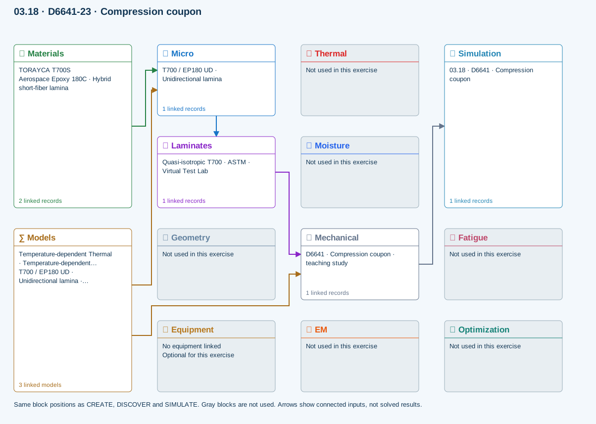
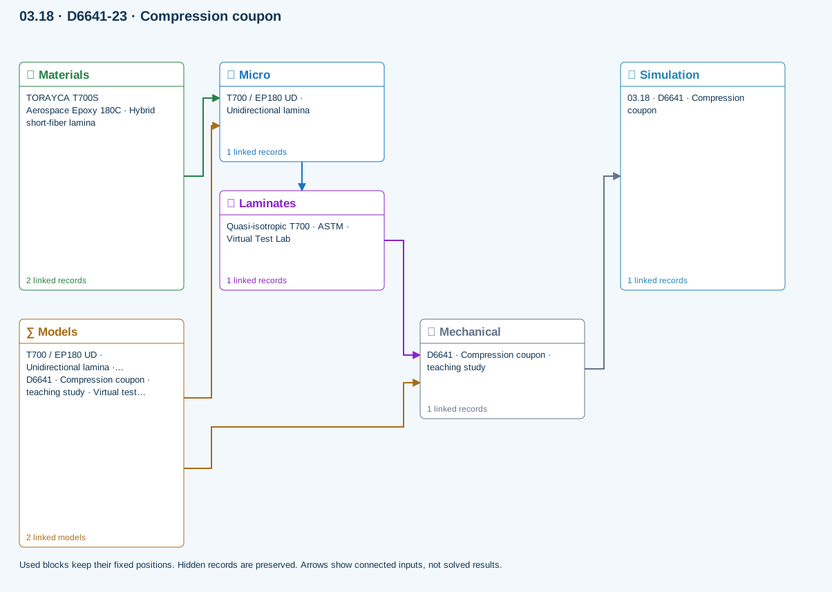
∑ Used models & submodels
Only models assigned to records used by this exercise are listed here. The full-layout option preserves the supplied starter records; no Workbench records are changed.
Halpin–Tsai · T700 / EP180 UD · Unidirectional lamina
One compatible homogenization model per Micro recipe. Separate recipes compare models; their predictions are not blended.
∑ Theory & assumptionsVirtual test · compression coupon · D6641 · Compression coupon · teaching study
Uniform small-strain compression using linked laminate Ex and thickness. Measured compressive strength supplies a screening ratio; fixture, tabs, buckling and failure evolution are not simulated.
Linked laminate reference state
Ply stiffness, thickness and orientation come from the linked laminate. Other thermal or structural analyses must be run separately.
Calibration & study controls
Teaching example
Specimen width: 25 mm
Gauge length: 25 mm
Applied force: 1000 N
Positive magnitude. Compression is reported as a magnitude.
Measured compressive strength: 400 MPa
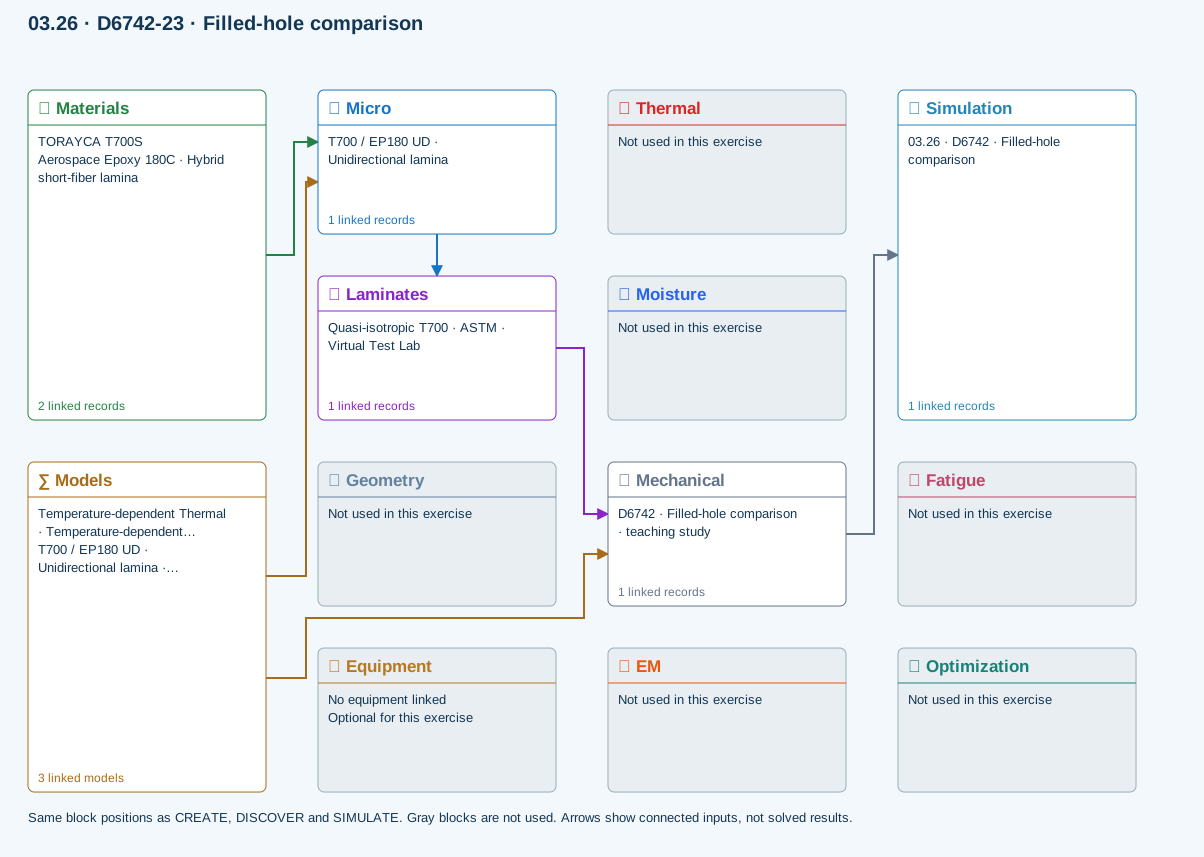
Data travelling between blocks
Micro → Laminates
Predicted ply stiffness, strength, density and expansion properties.
Materials → Micro
Constituent stiffness, strength, density and thermal / moisture properties.
Mechanical → Simulation
SIMULATION selects this case and its analysis model; the case owns its applicable cycle and input references.
Laminates → Mechanical
Ply angles and thicknesses, stiffness, mass and ply properties.
Models → Micro
Applied model assignment: Halpin–Tsai. Model parameters and formulation are used by Micro.
Models → Mechanical
Applied model assignment: Virtual test · compression coupon. Model parameters and formulation are used by Mechanical.
D5379-19(2026) / D7078-20(2025) · Shear coupon
Uniform nominal shear between notches using linked laminate Gxy and thickness. Not a notch/fixture stress field or nonlinear shear solution. Gauge length is the effective shear deformation length, not crosshead travel.
Equations, inputs and interpretation
τ = P/(bnet t), γ = τ/Gxy, δ = γLg.
Gxy and thickness come from the connected laminate. This uniform nominal-field approximation does not resolve the V-notch or grip stresses. Lg is an effective shear gauge length, not fixture travel. Supply measured shear strength separately. Both D5379 and D7078 are represented only at this nominal-response level.
- Net section width (mm)
- Shear gauge length (mm)
- Applied force (N)
- Measured shear strength (MPa)
Connected workflow
All blocks keep the CREATE / DISCOVER / SIMULATE positions, with Equipment below Geometry; unused records remain disconnected. This changes the view only, not the exercise records.
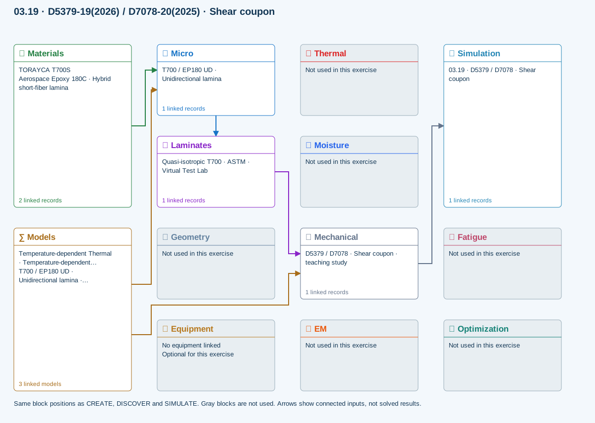
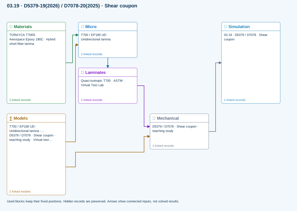
∑ Used models & submodels
Only models assigned to records used by this exercise are listed here. The full-layout option preserves the supplied starter records; no Workbench records are changed.
Halpin–Tsai · T700 / EP180 UD · Unidirectional lamina
One compatible homogenization model per Micro recipe. Separate recipes compare models; their predictions are not blended.
∑ Theory & assumptionsVirtual test · nominal shear coupon · D5379 / D7078 · Shear coupon · teaching study
Uniform nominal shear between notches using linked laminate Gxy and thickness. Not a notch/fixture stress field or nonlinear shear solution. Gauge length is the effective shear deformation length, not crosshead travel.
Linked laminate reference state
Ply stiffness, thickness and orientation come from the linked laminate. Other thermal or structural analyses must be run separately.
Calibration & study controls
Teaching example
Net section width: 12 mm
Shear gauge length: 10 mm
Applied force: 500 N
Measured shear strength: 80 MPa
Data travelling between blocks
Micro → Laminates
Predicted ply stiffness, strength, density and expansion properties.
Materials → Micro
Constituent stiffness, strength, density and thermal / moisture properties.
Mechanical → Simulation
SIMULATION selects this case and its analysis model; the case owns its applicable cycle and input references.
Laminates → Mechanical
Ply angles and thicknesses, stiffness, mass and ply properties.
Models → Micro
Applied model assignment: Halpin–Tsai. Model parameters and formulation are used by Micro.
Models → Mechanical
Applied model assignment: Virtual test · nominal shear coupon. Model parameters and formulation are used by Mechanical.
D5528-21 · DCB opening
Ideal Euler–Bernoulli DCB with equal homogeneous 0° arms, each half the linked laminate thickness. No root rotation, shear, large displacement or cohesive growth. Critical load is an initiation estimate from supplied GIc.
Equations, inputs and interpretation
C = 8a³/(Ebh³), GI = 12P²a²/(Eb²h³), Pc = √[GIc Eb²h³/(12a²)].
Each identical homogeneous 0° arm has thickness h = t/2. P is the force on each arm and δ = CP is relative opening. The linked ply E1 supplies the ideal beam modulus. Crack length stays fixed; Pc estimates initiation only. Root rotation, shear deformation, large deflection and compliance corrections required in experimental interpretation are absent. Use a/h ≥ 10.
- Specimen width (mm)
- Crack length (mm)
- Applied force (N)
- Critical fracture energy (N/mm)
Connected workflow
All blocks keep the CREATE / DISCOVER / SIMULATE positions, with Equipment below Geometry; unused records remain disconnected. This changes the view only, not the exercise records.
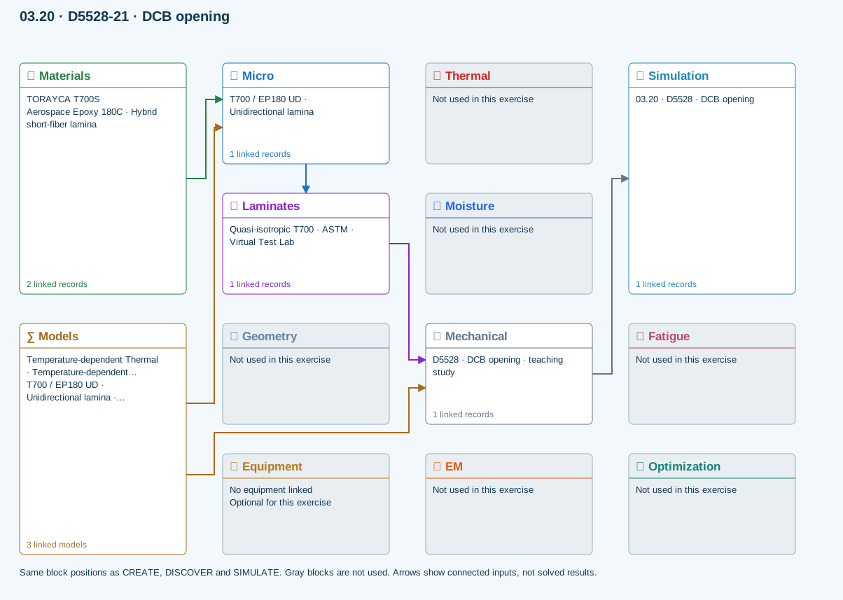
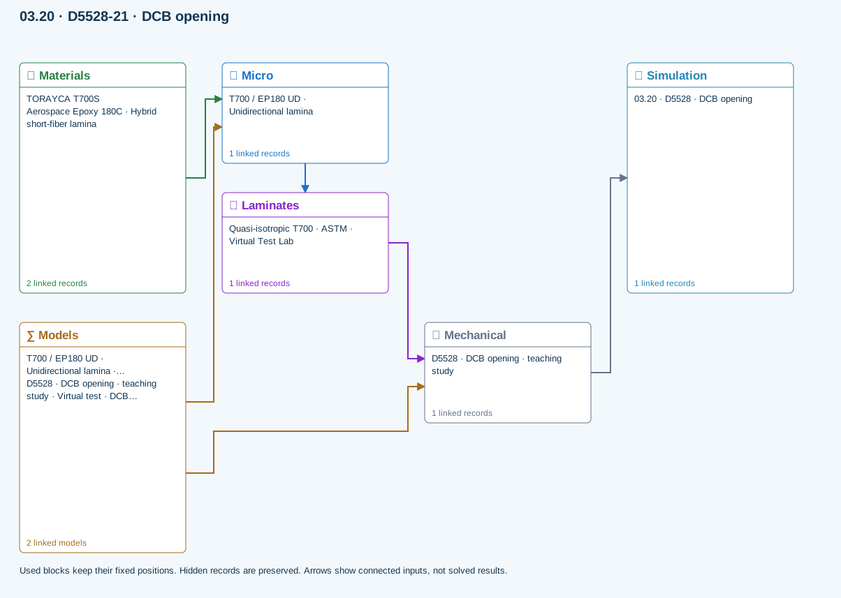
∑ Used models & submodels
Only models assigned to records used by this exercise are listed here. The full-layout option preserves the supplied starter records; no Workbench records are changed.
Halpin–Tsai · T700 / EP180 UD · Unidirectional lamina
One compatible homogenization model per Micro recipe. Separate recipes compare models; their predictions are not blended.
∑ Theory & assumptionsVirtual test · DCB beam compliance · D5528 · DCB opening · teaching study
Ideal Euler–Bernoulli DCB with equal homogeneous 0° arms, each half the linked laminate thickness. No root rotation, shear, large displacement or cohesive growth. Critical load is an initiation estimate from supplied GIc.
Linked laminate reference state
Ply stiffness, thickness and orientation come from the linked laminate. Other thermal or structural analyses must be run separately.
Calibration & study controls
Teaching example
Specimen width: 25 mm
Crack length: 30 mm
Applied force: 5 N
Critical fracture energy: 0.3 N/mm
Measured fracture energy; default is hypothetical.
Data travelling between blocks
Micro → Laminates
Predicted ply stiffness, strength, density and expansion properties.
Materials → Micro
Constituent stiffness, strength, density and thermal / moisture properties.
Mechanical → Simulation
SIMULATION selects this case and its analysis model; the case owns its applicable cycle and input references.
Laminates → Mechanical
Ply angles and thicknesses, stiffness, mass and ply properties.
Models → Micro
Applied model assignment: Halpin–Tsai. Model parameters and formulation are used by Micro.
Models → Mechanical
Applied model assignment: Virtual test · DCB beam compliance. Model parameters and formulation are used by Mechanical.
D7905-19e1 · ENF sliding
Ideal equal-arm, homogeneous 0° ENF beam; support span is twice the half-span. Crack must be shorter than the half-span. No shear/root correction or unstable crack growth. GIIc is supplied, not fitted automatically.
Equations, inputs and interpretation
C = (2L³ + 3a³)/(8Ebh³), GII = 9P²a²/(16Eb²h³).
L is the support HALF-span; each identical 0° arm has thickness h = t/2. The crack must satisfy a < L. At fixed crack length, δ = CP and the supplied GIIc determines the ideal initiation load. This is not an unstable crack-propagation simulation or a complete standard test reduction. Use slender beams.
- Specimen width (mm)
- Crack length (mm)
- Applied force (N)
- Critical fracture energy (N/mm)
- Support half-span (mm)
Connected workflow
All blocks keep the CREATE / DISCOVER / SIMULATE positions, with Equipment below Geometry; unused records remain disconnected. This changes the view only, not the exercise records.
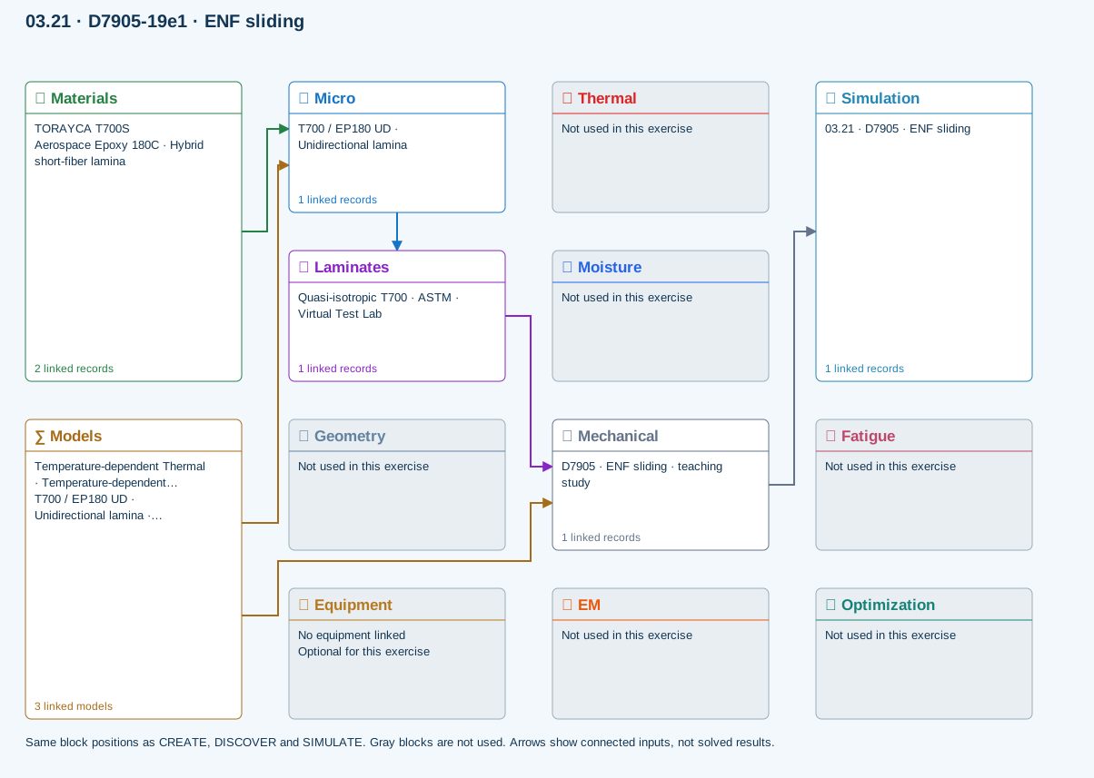
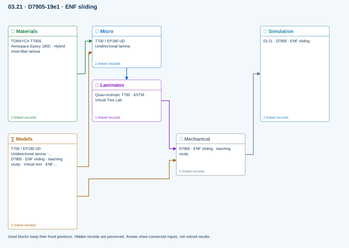
∑ Used models & submodels
Only models assigned to records used by this exercise are listed here. The full-layout option preserves the supplied starter records; no Workbench records are changed.
Halpin–Tsai · T700 / EP180 UD · Unidirectional lamina
One compatible homogenization model per Micro recipe. Separate recipes compare models; their predictions are not blended.
∑ Theory & assumptionsVirtual test · ENF beam compliance · D7905 · ENF sliding · teaching study
Ideal equal-arm, homogeneous 0° ENF beam; support span is twice the half-span. Crack must be shorter than the half-span. No shear/root correction or unstable crack growth. GIIc is supplied, not fitted automatically.
Linked laminate reference state
Ply stiffness, thickness and orientation come from the linked laminate. Other thermal or structural analyses must be run separately.
Calibration & study controls
Teaching example
Specimen width: 25 mm
Crack length: 30 mm
Applied force: 5 N
Critical fracture energy: 0.3 N/mm
Measured fracture energy; default is hypothetical.
Support half-span: 50 mm
Data travelling between blocks
Micro → Laminates
Predicted ply stiffness, strength, density and expansion properties.
Materials → Micro
Constituent stiffness, strength, density and thermal / moisture properties.
Mechanical → Simulation
SIMULATION selects this case and its analysis model; the case owns its applicable cycle and input references.
Laminates → Mechanical
Ply angles and thicknesses, stiffness, mass and ply properties.
Models → Micro
Applied model assignment: Halpin–Tsai. Model parameters and formulation are used by Micro.
Models → Mechanical
Applied model assignment: Virtual test · ENF beam compliance. Model parameters and formulation are used by Mechanical.
D6671-22 · Mixed-mode fracture envelope
Benzeggagh–Kenane envelope from calibrated GIc, GIIc and exponent. Supplied GI/GII are energy-release rates from a separate test reduction or analysis. This does not resolve the MMB lever fixture or propagate a crack.
Equations, inputs and interpretation
Gc = GIc + (GIIc − GIc) [GII/(GI + GII)]^η.
The BK envelope interpolates between measured pure-mode toughnesses using a calibrated exponent. The supplied GI and GII must come from an independent test reduction or compatible analysis. No lever-arm geometry or MMB fixture is solved. The laminate link keeps study provenance; laminate stiffness is not used to infer these energy-release rates.
- Mode I toughness (N/mm)
- Mode II toughness (N/mm)
- BK exponent (—)
- Applied GI (N/mm)
- Applied GII (N/mm)
Connected workflow
All blocks keep the CREATE / DISCOVER / SIMULATE positions, with Equipment below Geometry; unused records remain disconnected. This changes the view only, not the exercise records.
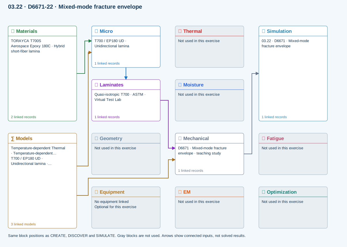
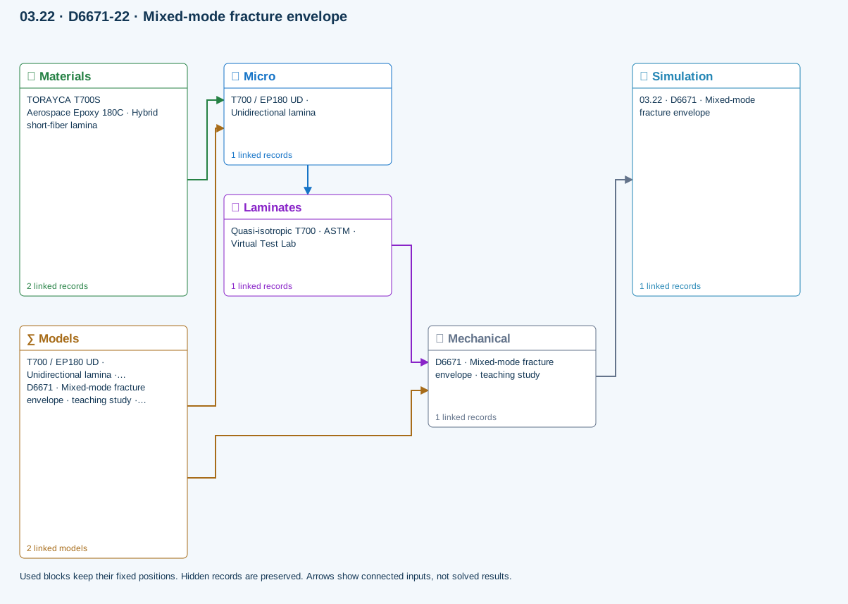
∑ Used models & submodels
Only models assigned to records used by this exercise are listed here. The full-layout option preserves the supplied starter records; no Workbench records are changed.
Halpin–Tsai · T700 / EP180 UD · Unidirectional lamina
One compatible homogenization model per Micro recipe. Separate recipes compare models; their predictions are not blended.
∑ Theory & assumptionsVirtual test · BK mixed-mode envelope · D6671 · Mixed-mode fracture envelope · teaching study
Benzeggagh–Kenane envelope from calibrated GIc, GIIc and exponent. Supplied GI/GII are energy-release rates from a separate test reduction or analysis. This does not resolve the MMB lever fixture or propagate a crack.
Linked laminate reference state
Ply stiffness, thickness and orientation come from the linked laminate. Other thermal or structural analyses must be run separately.
Calibration & study controls
Teaching example
Mode I toughness: 0.3 N/mm
Mode II toughness: 0.9 N/mm
BK exponent: 1.6 —
Applied GI: 0.1 N/mm
Applied GII: 0.2 N/mm
Data travelling between blocks
Micro → Laminates
Predicted ply stiffness, strength, density and expansion properties.
Materials → Micro
Constituent stiffness, strength, density and thermal / moisture properties.
Mechanical → Simulation
SIMULATION selects this case and its analysis model; the case owns its applicable cycle and input references.
Laminates → Mechanical
Ply angles and thicknesses, stiffness, mass and ply properties.
Models → Micro
Applied model assignment: Halpin–Tsai. Model parameters and formulation are used by Micro.
Models → Mechanical
Applied model assignment: Virtual test · BK mixed-mode envelope. Model parameters and formulation are used by Mechanical.
D5229-20 · Moisture uptake calibration
Homogeneous slab, initially dry, both faces held at equilibrium moisture. Fits diffusivity from two early uptake measurements (both ≤50% saturation) using the square-root-time approximation. Edge ingress and temperature dependence are excluded. Does not overwrite material properties.
Equations, inputs and interpretation
D = π [t × slope/(4M∞)]²; M(T)/M∞ = 1 − (8/π²) Σ exp[−(2j+1)²π²DT/t²]/(2j+1)².
Here t is total slab thickness and T is elapsed time. Two increasing early mass-gain points define slope = ΔM/Δ√T. Both must remain at or below 50% of equilibrium; an inconsistent dry intercept is rejected. The model assumes an initially dry homogeneous slab with both faces held at equilibrium, no edge ingress and constant diffusivity. D is reported in mm²/s. Copy it into a material only after independent validation; no saved material is changed. No temperature shifting or hot-wet strength degradation is inferred.
- Equilibrium mass gain (percent)
- Measurement time 1 (h)
- Mass gain 1 (percent)
- Measurement time 2 (h)
- Mass gain 2 (percent)
- Conditioning duration (h)
Connected workflow
All blocks keep the CREATE / DISCOVER / SIMULATE positions, with Equipment below Geometry; unused records remain disconnected. This changes the view only, not the exercise records.
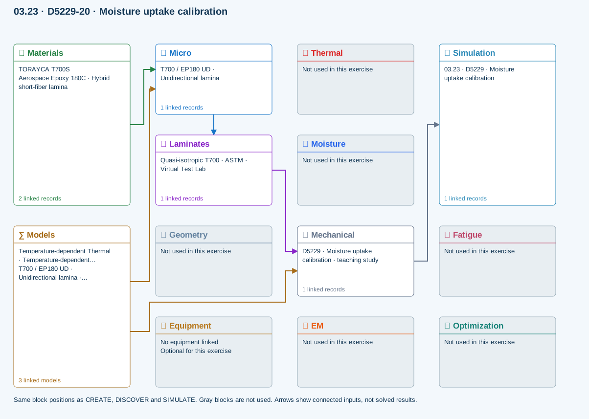
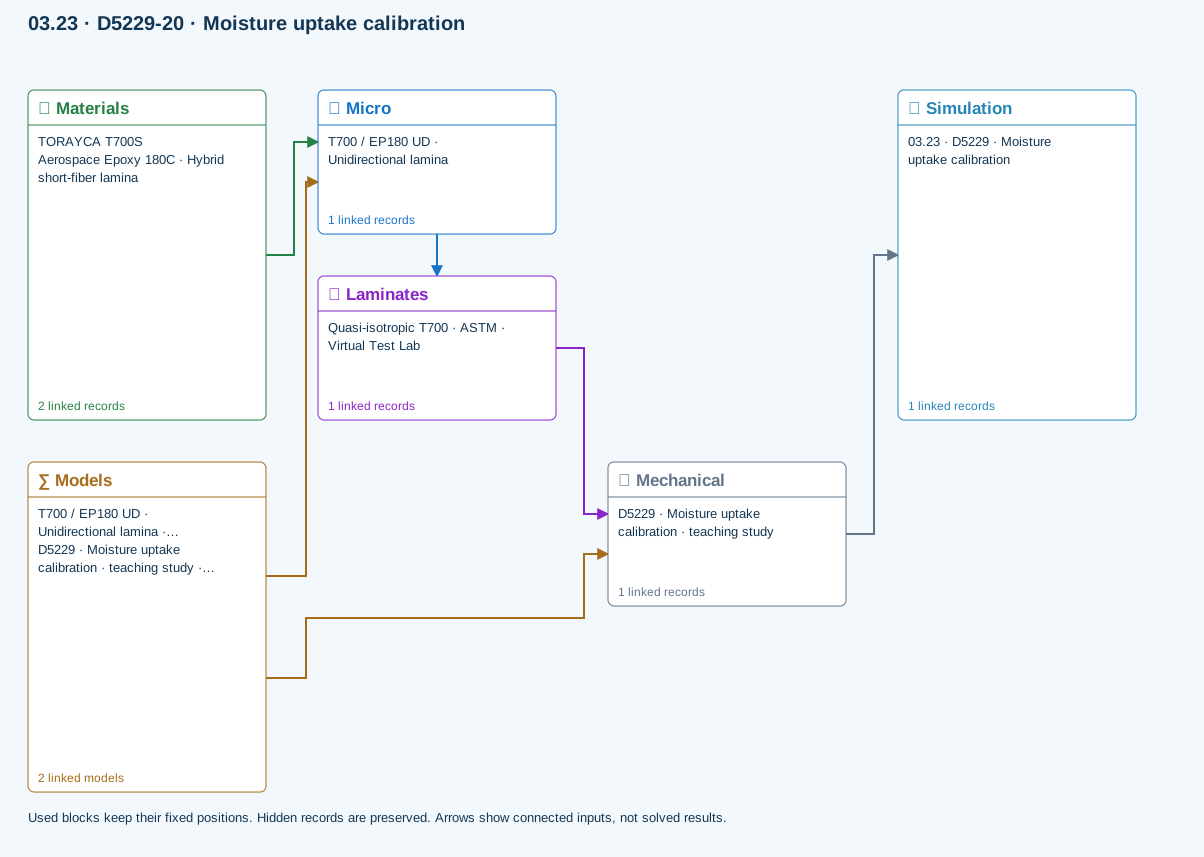
∑ Used models & submodels
Only models assigned to records used by this exercise are listed here. The full-layout option preserves the supplied starter records; no Workbench records are changed.
Halpin–Tsai · T700 / EP180 UD · Unidirectional lamina
One compatible homogenization model per Micro recipe. Separate recipes compare models; their predictions are not blended.
∑ Theory & assumptionsVirtual test · Fickian uptake calibration · D5229 · Moisture uptake calibration · teaching study
Homogeneous slab, initially dry, both faces held at equilibrium moisture. Fits diffusivity from two early uptake measurements (both ≤50% saturation) using the square-root-time approximation. Edge ingress and temperature dependence are excluded. Does not overwrite material properties.
Linked laminate reference state
Ply stiffness, thickness and orientation come from the linked laminate. Other thermal or structural analyses must be run separately.
Calibration & study controls
Teaching example
Equilibrium mass gain: 1 percent
Measurement time 1: 1 h
Mass gain 1: 0.05 percent
Measurement time 2: 4 h
Mass gain 2: 0.1 percent
Conditioning duration: 100 h
Data travelling between blocks
Micro → Laminates
Predicted ply stiffness, strength, density and expansion properties.
Materials → Micro
Constituent stiffness, strength, density and thermal / moisture properties.
Mechanical → Simulation
SIMULATION selects this case and its analysis model; the case owns its applicable cycle and input references.
Laminates → Mechanical
Ply angles and thicknesses, stiffness, mass and ply properties.
Models → Micro
Applied model assignment: Halpin–Tsai. Model parameters and formulation are used by Micro.
Models → Mechanical
Applied model assignment: Virtual test · Fickian uptake calibration. Model parameters and formulation are used by Mechanical.
D5961-23 · Bearing / bypass screening
Single-pin nominal bearing, net-section and shear-out checks with independent measured allowables. Bypass tension is added to net-section load only. No contact, bolt preload, load redistribution or validated bearing–bypass interaction envelope.
Equations, inputs and interpretation
σbearing = P/(dt); σnet = (P + Pbypass)/[(w − d)t]; τout = P/[2(e − d/2)t].
e is the hole-center distance to the loaded free edge. Each nominal stress is compared with its own measured allowable. Bypass tension contributes to the net-section load. These independent ratios are not a validated bearing–bypass interaction surface. Bolt preload, contact, friction, multi-fastener load sharing and progressive damage require further modeling.
- Specimen width (mm)
- Hole diameter (mm)
- Edge distance (mm)
- Pin force (N)
- Bypass tensile force (N)
- Bearing allowable (MPa)
- Net tensile allowable (MPa)
- Shear-out allowable (MPa)
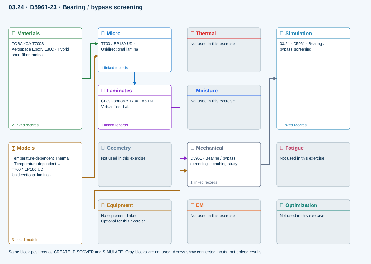
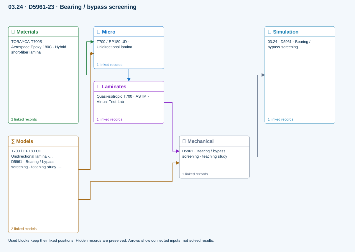
Connected workflow
All blocks keep the CREATE / DISCOVER / SIMULATE positions, with Equipment below Geometry; unused records remain disconnected. This changes the view only, not the exercise records.
∑ Used models & submodels
Only models assigned to records used by this exercise are listed here. The full-layout option preserves the supplied starter records; no Workbench records are changed.
Halpin–Tsai · T700 / EP180 UD · Unidirectional lamina
One compatible homogenization model per Micro recipe. Separate recipes compare models; their predictions are not blended.
∑ Theory & assumptionsVirtual test · bearing bypass screening · D5961 · Bearing / bypass screening · teaching study
Single-pin nominal bearing, net-section and shear-out checks with independent measured allowables. Bypass tension is added to net-section load only. No contact, bolt preload, load redistribution or validated bearing–bypass interaction envelope.
Linked laminate reference state
Ply stiffness, thickness and orientation come from the linked laminate. Other thermal or structural analyses must be run separately.
Calibration & study controls
Teaching example
Specimen width: 36 mm
Hole diameter: 6 mm
Edge distance: 18 mm
Hole center to loaded free edge.
Pin force: 1000 N
Bypass tensile force: 500 N
Bearing allowable: 300 MPa
Net tensile allowable: 400 MPa
Shear-out allowable: 80 MPa
Data travelling between blocks
Micro → Laminates
Predicted ply stiffness, strength, density and expansion properties.
Materials → Micro
Constituent stiffness, strength, density and thermal / moisture properties.
Mechanical → Simulation
SIMULATION selects this case and its analysis model; the case owns its applicable cycle and input references.
Laminates → Mechanical
Ply angles and thicknesses, stiffness, mass and ply properties.
Models → Micro
Applied model assignment: Halpin–Tsai. Model parameters and formulation are used by Micro.
Models → Mechanical
Applied model assignment: Virtual test · bearing bypass screening. Model parameters and formulation are used by Mechanical.
D6484-23 · Open-hole compression
Nominal gross/net stress and demand relative to measured open-hole compressive strength for this geometry and layup. This is test-data screening, not an uncalibrated notch-strength prediction. No local buckling or kink-band simulation.
Equations, inputs and interpretation
σgross = P/(wt); σnet = P/[(w − d)t]; demand = σgross/XOHC.
XOHC is the measured gross-section compressive strength for this layup and hole geometry. Do not compare net stress with a gross-section allowable. This assessment does not reuse the Whitney–Nuismer tension model or predict compressive notch strength.
- Specimen width (mm)
- Hole diameter (mm)
- Applied force (N)
- Measured open-hole compressive strength (MPa)
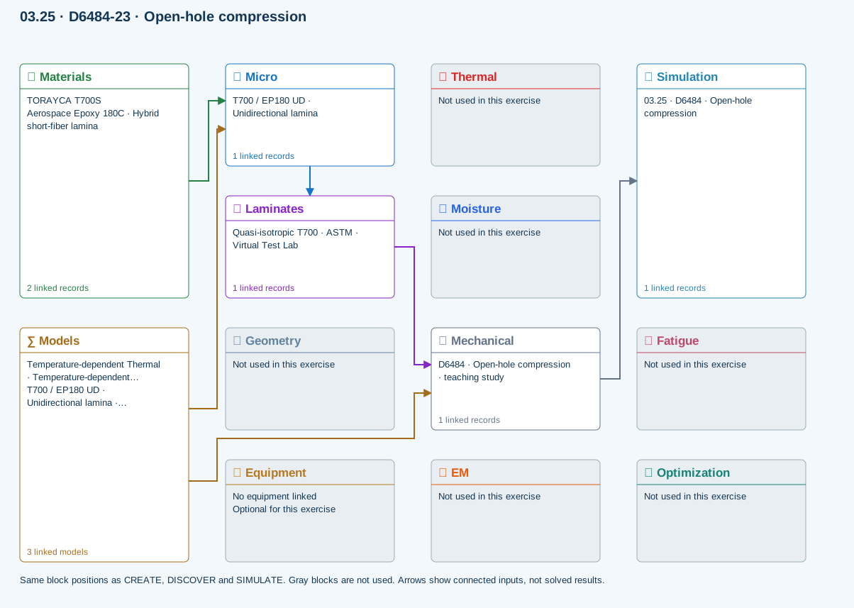
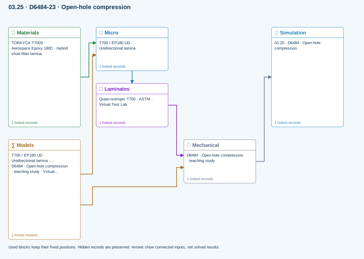
Connected workflow
All blocks keep the CREATE / DISCOVER / SIMULATE positions, with Equipment below Geometry; unused records remain disconnected. This changes the view only, not the exercise records.
∑ Used models & submodels
Only models assigned to records used by this exercise are listed here. The full-layout option preserves the supplied starter records; no Workbench records are changed.
Halpin–Tsai · T700 / EP180 UD · Unidirectional lamina
One compatible homogenization model per Micro recipe. Separate recipes compare models; their predictions are not blended.
∑ Theory & assumptionsVirtual test · measured open-hole compression · D6484 · Open-hole compression · teaching study
Nominal gross/net stress and demand relative to measured open-hole compressive strength for this geometry and layup. This is test-data screening, not an uncalibrated notch-strength prediction. No local buckling or kink-band simulation.
Linked laminate reference state
Ply stiffness, thickness and orientation come from the linked laminate. Other thermal or structural analyses must be run separately.
Calibration & study controls
Teaching example
Specimen width: 36 mm
Hole diameter: 6 mm
Applied force: 1000 N
Measured open-hole compressive strength: 250 MPa
Data travelling between blocks
Micro → Laminates
Predicted ply stiffness, strength, density and expansion properties.
Materials → Micro
Constituent stiffness, strength, density and thermal / moisture properties.
Mechanical → Simulation
SIMULATION selects this case and its analysis model; the case owns its applicable cycle and input references.
Laminates → Mechanical
Ply angles and thicknesses, stiffness, mass and ply properties.
Models → Micro
Applied model assignment: Halpin–Tsai. Model parameters and formulation are used by Micro.
Models → Mechanical
Applied model assignment: Virtual test · measured open-hole compression. Model parameters and formulation are used by Mechanical.
D6742-23 · Filled-hole comparison
Compares user-measured open- and filled-hole compressive strengths using gross-section stress. Use matched layup, hole, environment and fastener condition. Filling a hole does not automatically recover strength; no fastener contact/preload model is applied.
Equations, inputs and interpretation
Demandopen = σgross/XOHC; Demandfilled = σgross/XFHC.
Compare matched measured open- and filled-hole compressive strengths. Pin fit, preload, environment and geometry must match the calibration basis. Filling the hole is not assumed to restore strength, and the curves show nominal demand scaling rather than predicted damage or load–deflection.
- Specimen width (mm)
- Hole diameter (mm)
- Applied force (N)
- Measured open-hole compressive strength (MPa)
- Measured filled-hole compressive strength (MPa)
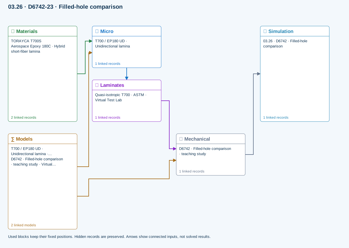
Connected workflow
All blocks keep the CREATE / DISCOVER / SIMULATE positions, with Equipment below Geometry; unused records remain disconnected. This changes the view only, not the exercise records.
∑ Used models & submodels
Only models assigned to records used by this exercise are listed here. The full-layout option preserves the supplied starter records; no Workbench records are changed.
Halpin–Tsai · T700 / EP180 UD · Unidirectional lamina
One compatible homogenization model per Micro recipe. Separate recipes compare models; their predictions are not blended.
∑ Theory & assumptionsVirtual test · measured filled-hole comparison · D6742 · Filled-hole comparison · teaching study
Compares user-measured open- and filled-hole compressive strengths using gross-section stress. Use matched layup, hole, environment and fastener condition. Filling a hole does not automatically recover strength; no fastener contact/preload model is applied.
Linked laminate reference state
Ply stiffness, thickness and orientation come from the linked laminate. Other thermal or structural analyses must be run separately.
Calibration & study controls
Teaching example
Specimen width: 36 mm
Hole diameter: 6 mm
Applied force: 1000 N
Measured open-hole compressive strength: 250 MPa
Measured filled-hole compressive strength: 300 MPa
Data travelling between blocks
Micro → Laminates
Predicted ply stiffness, strength, density and expansion properties.
Materials → Micro
Constituent stiffness, strength, density and thermal / moisture properties.
Mechanical → Simulation
SIMULATION selects this case and its analysis model; the case owns its applicable cycle and input references.
Laminates → Mechanical
Ply angles and thicknesses, stiffness, mass and ply properties.
Models → Micro
Applied model assignment: Halpin–Tsai. Model parameters and formulation are used by Micro.
Models → Mechanical
Applied model assignment: Virtual test · measured filled-hole comparison. Model parameters and formulation are used by Mechanical.
D7136-25 / D7137-23 · Impact & CAI assessment
Incident energy from measured impact velocity; residual compressive strength from measured peak CAI force. Rebound energy estimates energy not returned to the striker, NOT damage energy. No impact/contact solver, damage-area prediction or energy-to-strength extrapolation.
Equations, inputs and interpretation
Eincident = mv²/2; Erebound = mvr²/2; XCAI = Ppeak/(wt).
Enter measured impact and rebound velocities, measured CAI peak force and pristine compressive strength. Energy not returned to the striker includes mechanisms other than damage. The strength-retention ratio is a measured comparison, not an energy-to-strength prediction. No synthetic impact pulse, damage footprint or full-wave impact solution is generated.
- Impactor mass (kg)
- Impact speed (m/s)
- Rebound speed (m/s)
- Specimen width (mm)
- Measured CAI peak force (N)
- Measured pristine compressive strength (MPa)
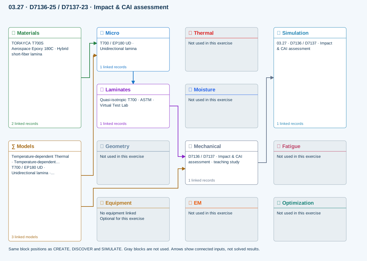
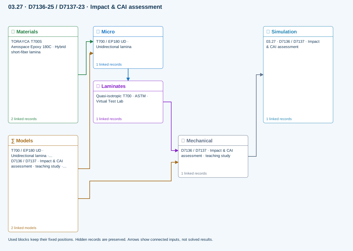
Connected workflow
All blocks keep the CREATE / DISCOVER / SIMULATE positions, with Equipment below Geometry; unused records remain disconnected. This changes the view only, not the exercise records.
∑ Used models & submodels
Only models assigned to records used by this exercise are listed here. The full-layout option preserves the supplied starter records; no Workbench records are changed.
Halpin–Tsai · T700 / EP180 UD · Unidirectional lamina
One compatible homogenization model per Micro recipe. Separate recipes compare models; their predictions are not blended.
∑ Theory & assumptionsVirtual test · measured impact and CAI · D7136 / D7137 · Impact & CAI assessment · teaching study
Incident energy from measured impact velocity; residual compressive strength from measured peak CAI force. Rebound energy estimates energy not returned to the striker, NOT damage energy. No impact/contact solver, damage-area prediction or energy-to-strength extrapolation.
Linked laminate reference state
Ply stiffness, thickness and orientation come from the linked laminate. Other thermal or structural analyses must be run separately.
Calibration & study controls
Teaching example
Impactor mass: 5 kg
Impact speed: 2 m/s
Rebound speed: 0.5 m/s
Specimen width: 100 mm
Measured CAI peak force: 30000 N
Measured pristine compressive strength: 400 MPa
Data travelling between blocks
Micro → Laminates
Predicted ply stiffness, strength, density and expansion properties.
Materials → Micro
Constituent stiffness, strength, density and thermal / moisture properties.
Mechanical → Simulation
SIMULATION selects this case and its analysis model; the case owns its applicable cycle and input references.
Laminates → Mechanical
Ply angles and thicknesses, stiffness, mass and ply properties.
Models → Micro
Applied model assignment: Halpin–Tsai. Model parameters and formulation are used by Micro.
Models → Mechanical
Applied model assignment: Virtual test · measured impact and CAI. Model parameters and formulation are used by Mechanical.