
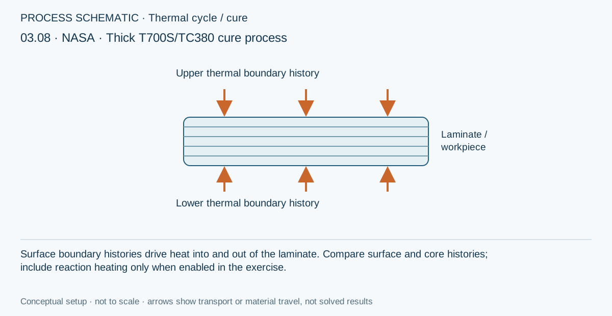
A process history specifies how the environment changes, while the solved material state may differ from that environment. Thermal lag, reaction heat and moisture uptake depend on the selected constitutive and transport models. Inspect the initial state and each exposed or constrained surface before running a transient study, and identify which resulting fields are transferred to a later calculation.
Connect reusable Equipment before comparing line designs. A heater die and cooling die each own dimensions and thermal settings; the thermal case places them against the Upper or Lower surface. Check the contact footprint in Live Process and preserve the linked hardware with the simulation.
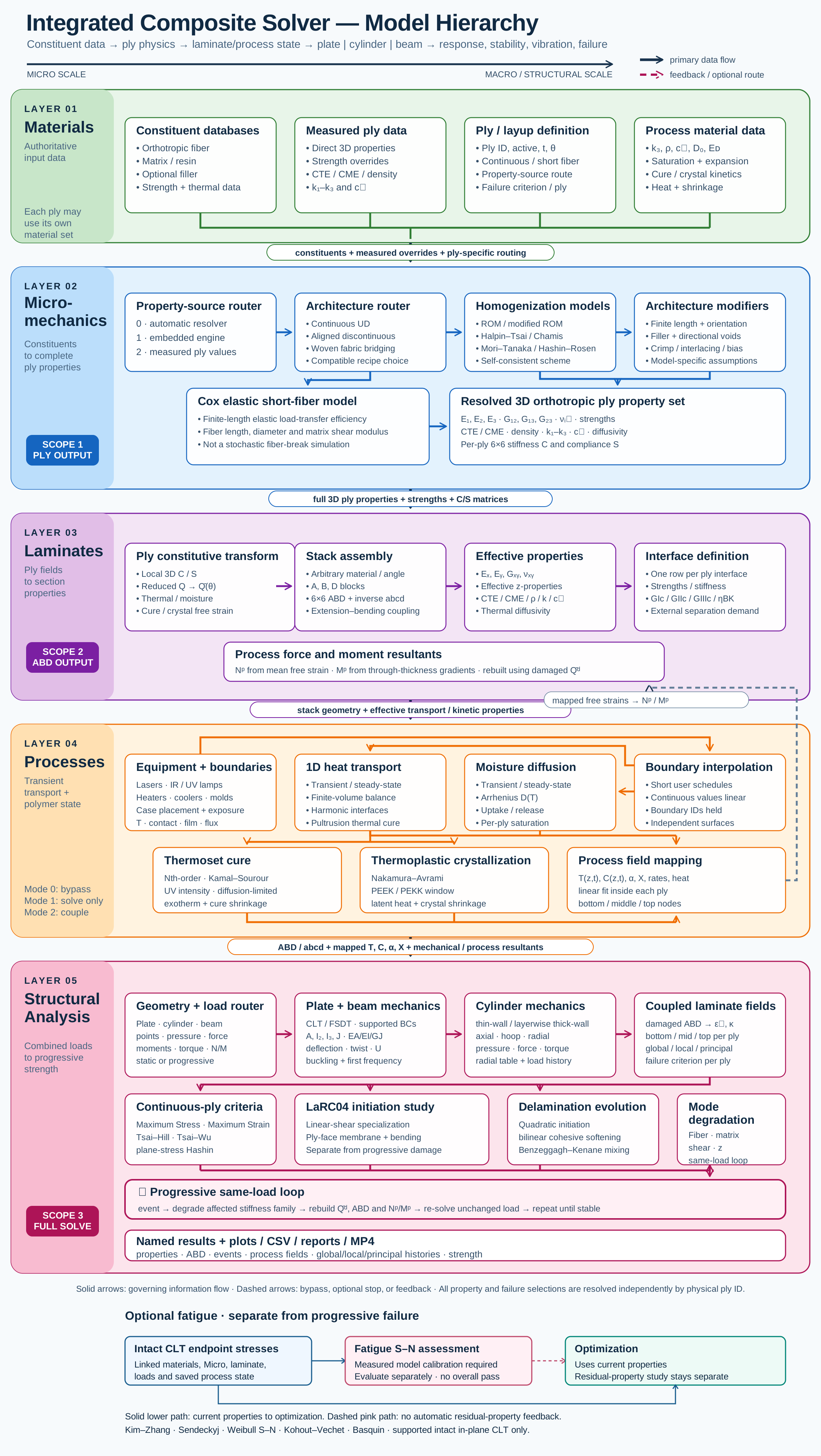
5.1 Connect design intent to process behavior.
Workflow / 03.4 Processing
Solve steady-state or transient through-thickness process response before structural analysis, using effective ply transport properties, independent top and bottom schedules, cure exotherm, cure-dependent modulus, polymer kinetics, water uptake or release, and process-cycle optimization.
Connected model layer
Processing model map
Select a block to explore its theory or workflow. View the complete Model Map
Equipment is part of the connected study
Pultrusion now uses linked heating and cooling dies with explicit contact intervals. Open the die setup and thermal-contact guide for placement, equations, example settings and limits.
Equipment stays directly below Geometry in CREATE, DISCOVER and SIMULATE. Select reusable lasers, IR/UV lamps, heaters, coolers or molds, then connect them to the applicable thermal boundary. Equipment owns hardware dimensions, power or temperature, contact conductance, vendor and surface-material details; the case owns position, angle, side and exposure timing.
Changing a hardware record updates every boundary using it. Duplicate it first when a change should apply to only one installation. Rollers retain their Geometry records. A convection boundary can remain a prescribed environment without an Equipment record.
Explore the multi-zone pultrusion exercise →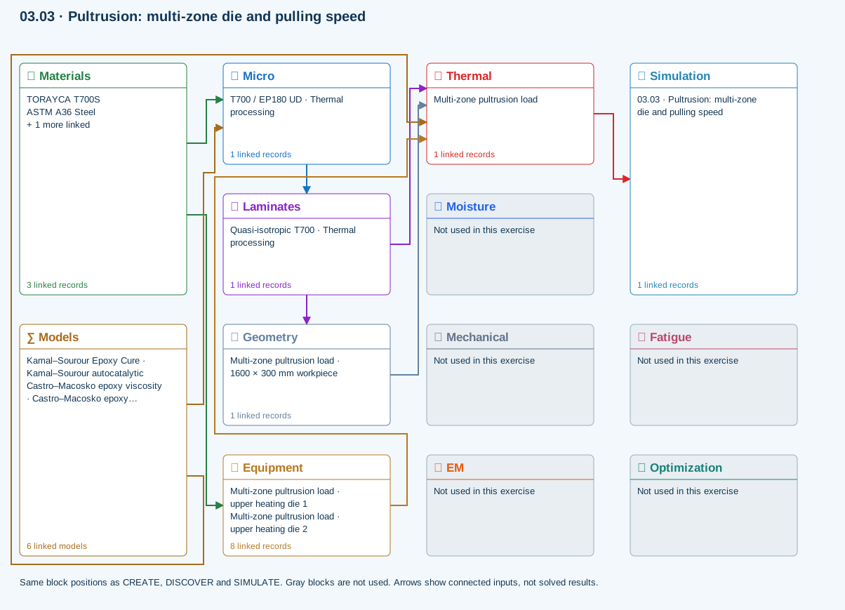
03.62 · Thick laminate: reaction heating, cure gradient and process stress
Level 4AdvancedEst. 40 min
Only blocks on the exercise path are shown. This changes the view only, not the exercise records.
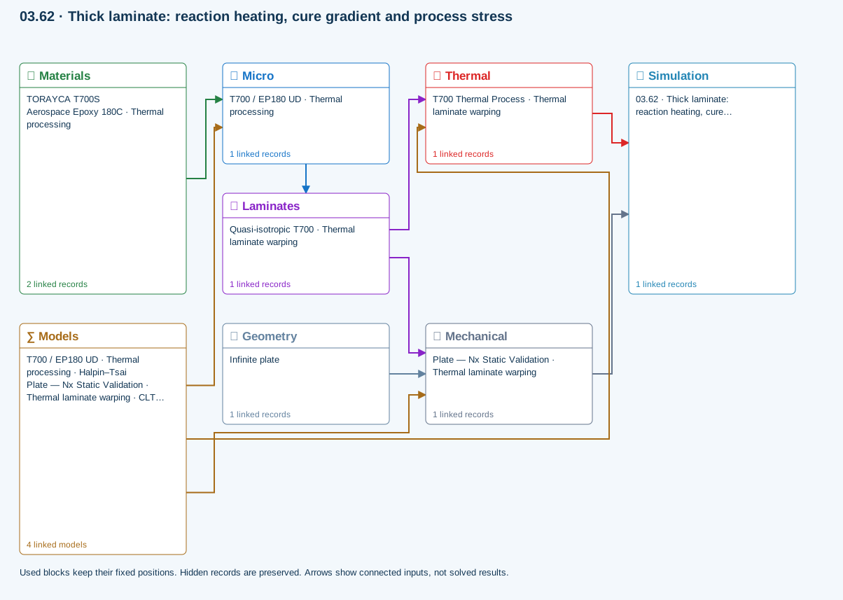
∑ Used models & submodels
Only models assigned to records used by this exercise are listed here. The full-layout option preserves the supplied starter records; no Workbench records are changed.
Halpin–Tsai · T700 / EP180 UD · Thermal processing
One compatible homogenization model per Micro recipe. Separate recipes compare models; their predictions are not blended.
∑ Theory & assumptionsCLT · Linear static with failure indices · Plate — Nx Static Validation · Thermal laminate warping
Shared laminate stiffness drives this membrane/CLT path. Failure criteria are independent comparisons, not blended models. Fatigue is a separate assessment.
∑ Theory & assumptions1D transient heat transfer · T700 Thermal Process · Thermal laminate warping
Needs linked laminate properties and a compatible process schedule. A linked cycle is not a solved temperature history.
∑ Theory & assumptionsMaximum stress · Plate — Nx Static Validation · Thermal laminate warping
Primary ply criterion for Plate — Nx Static Validation · Thermal laminate warping. Envelope comparisons are independent; criteria are not blended.
∑ Theory & assumptionsData travelling between blocks
Micro → Laminates
Predicted ply stiffness, strength, density and expansion properties.
Materials → Micro
Constituent stiffness, strength, density and thermal / moisture properties.
Mechanical → Simulation
SIMULATION selects this case and its analysis model; the case owns its applicable cycle and input references.
Laminates → Mechanical
Ply angles and thicknesses, stiffness, mass and ply properties.
Geometry → Mechanical
Part shape and dimensions, thickness or section definition, and model-specific geometric inputs. Each selected case consumes only the dimensions its model supports.
Thermal → Simulation
SIMULATION selects this case and its analysis model; the case owns its applicable cycle and input references.
Laminates → Thermal
Ply angles and thicknesses, stiffness, mass and ply properties.
Models → Micro
Applied model assignment: Halpin–Tsai. Model parameters and formulation are used by Micro.
Models → Mechanical
Applied model assignment: CLT · Linear static with failure indices. Model parameters and formulation are used by Mechanical.; Maximum stress
Models → Thermal
Applied model assignment: 1D transient heat transfer. Model parameters and formulation are used by Thermal.
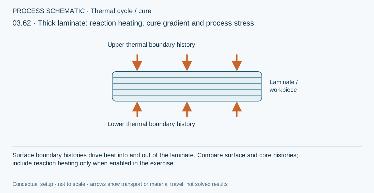
Run the 6 mm laminate through the 120°C dwell with its linked resin reaction heat.
Models: Heat transfer · Classical laminate theory · Extension–bending coupling · Thermomechanical coupling
Study scope and limitations
Teaching inputs, not qualified allowables. Sequential coupling transfers the reported thermal/moisture state to laminate mechanics; it is not simultaneous 3D multiphysics. Inspect the transferred state and reference values before interpreting stress or curvature. Free laminate CLT curvature, not fixture-constrained distortion, a full tool-release simulation or calibrated cure-shrinkage prediction.
03.4 / Workflow focus
Connected engineering recordIndependent boundary schedules
Thermal and moisture loads each need compatible material properties, a laminate, initial conditions and their own surface schedule.
Thermal and moisture formulations
Choose the steady or transient transport model for the study. Transient histories resolve the supported one-dimensional through-thickness problem.
Cure, crystallization and UV
Assigned calibrated material laws govern supported polymer-state calculations. UV cure needs its exposure inputs; pultrusion needs the distance/time relationship and pulling speed.
Supported coupling
A process schedule alone is not a solved history. Only compatible coupled analyses consume recovered environmental fields; reference-elastic studies remain separate.
Tool-release shape
The separate free-release CLT study uses prescribed temperatures and effective shrinkage. It is not a tool-contact simulation or an automatic transfer of the thermal cure history.
Process optimization
Compare bounded cycle candidates under supported objectives, save the validation data and rerun the selected candidate.
Use this workflow in Workbench: interactive Blocks, record selections and connection controls →
Connected model layer
Processing · released model connections
Select a model family to follow its inputs, results, theory and exercise. All model families ↗
Follow the connections
Heat, moisture & manufacturing
Material laws & boundary cycles
Calibrated kinetics, modulus or transport laws and material assignment
Transport & reaction
History & compatible process fields
Material laws consumed by compatible Micro or transport calculations
Representative exercise: this map shows its supplied records and active connections, not every possible configuration of the model family.
Only blocks on the exercise path are shown. This changes the view only, not the exercise records.
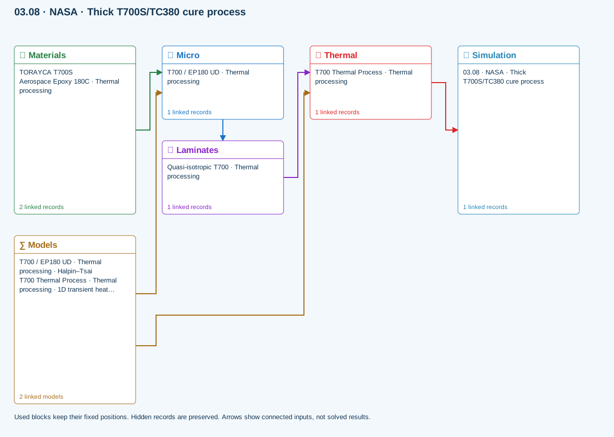
Cure, crystallization & material transport
Independent model records can be linked together through material inputs. A saved model must be assigned to a material before it contributes to a simulation.
Model choices and Workbench location
Models → material-model folders · assigned through Materials
- Kamal–Sourour autocatalytic
- Kamal–Sourour with diffusion control
- Nth-order Arrhenius
- CHILE (degree of cure)
- UV intensity-dependent cure
- Nakamura–Avrami
- Temperature-dependent tabular
- 1D Fickian diffusion
5.2 Pultrusion heating and cooling dies
06.1 Manuals · read online, preview or download →
Processing / Equipment
Use linked Equipment records to define the stationary tools around a moving composite section. The thermal solver predicts the material temperature and cure history as it passes through their contact footprints.
Separate the tool from its installation
A Heater or Cooler record owns contact length, width, body thickness, thermal control, body temperature or signed surface heat flux, and contact conductance. It also stores manufacturer, part number, specification source, body material, surface finish material and finish details. The thermal case links that record and owns its Upper or Lower placement and enabled state. Multiple placements can share one record; duplicate the hardware when its settings should vary independently.
Equipment is below Geometry in the fixed workflow. Rollers remain Geometry records. A heating die is a Heater installation and a cooling die is a Cooler installation. These are rectangular thermal-contact bodies; their name does not add die-cavity geometry, resin-flow or pulling-force physics.
Locate contact from the inlet surface
The Live Process origin is the width centre of the inlet upper surface. Positive x follows travel, y spans width and z is normal to the upper surface. Tool x is its centre; a tool of contact length L covers x minus L/2 to x plus L/2. Upper contact is at z = 0; lower contact is at minus the laminate thickness. Tools remain centred across the width. Seat them on the surface using the grid and snap controls. A lifted tool contributes no contact heat.
Choose Contact equipment on the appropriate boundary and link or place the tool. The active footprint is determined by the seated body, not by changing the composite to a prescribed temperature. Dragging the tool changes its installation; double-clicking opens the linked hardware record. Select Upper or Lower to see that domain's markers and click a marker to find its table row.
Finite contact exchange
For prescribed tool temperature, heat flows into the composite according to the difference between tool temperature and the current solved surface temperature:
q″ = hc (Tdie − Tsurface)
Here q″ is inward heat flux in W/m², hc is contact conductance in W/(m² K), and temperatures may be in °C when used as a difference. A 150°C die does not instantly impose 150°C on every ply. The material surface and core may lag the tool; enabled cure exotherm can also raise the material above a setpoint. A lower die setpoint removes heat when the surface is hotter than the tool.
Surface heat flux instead prescribes q″ directly: positive adds heat and negative removes it. Do not interpret this mode as temperature control or a prediction of electrical heater power. Contact width smaller than the part width is averaged over the modelled width, with the uncovered portion retaining its background condition. Same-side overlapping seated contact bodies are rejected rather than counted twice.
Convert line position to residence time
At constant speed v, elapsed residence time is x/v. If x is in metres and v is in m/min, time is in minutes. Each contact edge becomes a boundary event in the thermal integration. Step rows hold their value until the next station; Ramp rows interpolate eligible boundary values. The example dies use explicit constant intervals so a cooling region cannot be swallowed by the preceding hot zone.
| Example | Heating die intervals | Cooling die interval | Residence at 0.1 m/min |
|---|---|---|---|
| Heated and cooled starter | 0–0.8 m at 150°C | 0.8–1.0 m at 40°C | 10 min |
| Multi-zone pultrusion | 0–0.4 m at 80°C; 0.4–1.0 m at 150°C; 1.0–1.4 m at 180°C | 1.4–1.6 m at 40°C | 16 min |
Both faces use separate die installations, a 300 mm illustrative width and 500 W/(m² K) contact conductance. Initial material temperature is 23°C. These editable teaching settings are not qualified production recipes. Use Review library updates to replace old examples and dependencies without overwriting custom work.
Evaluate the process and its limits
Run the active simulation, then compare surface and core temperatures, through-thickness gradients, cure state and reaction heat against axial position. Change pulling speed, contact length, conductance or setpoint one at a time. Review the connected laminate and its cure, viscosity and modulus models before interpreting a process-to-structure transfer. Quality outputs exist only for enabled compatible models; a cured-looking temperature plot does not prove impregnation or low void content.
The moving-section thermal model resolves through-thickness conduction and enabled reaction sources. It excludes axial conduction, die thermal mass and internal temperature gradients, coolant circuits, feedback control, die friction, pulling load and general resin flow. Body and finish material selections document the tool; they do not derive contact conductance or solve heat storage in the die. A prescribed tool temperature represents a controlled boundary. Predicting die warm-up or repeated-pass die temperature requires a separate conjugate tool model.
Open the multi-zone pultrusion exercise · Follow the Equipment workflow
Chapter review
Keep environmental conditions, solved fields and mechanical reference states distinct in the saved study.
Current Workbench model references
These model-specific guides describe the documented Workbench controls. Read their calibration requirements and coupling limits; release notes distinguish announced releases from development previews.
References and source sections
References are retained with the formulations they support. Software instructions describe implementation scope; a cited source does not establish independent validation of a CDS calculation.