
Processing predicts the material history rather than simply prescribing the oven or die temperature to every ply. Heat conduction, boundary transfer and internal heat generation jointly determine the temperature field. Cure or crystallization can feed heat back into that field when the selected coupled model supports the reaction source.
Initial temperature is a material state. Surface schedules describe prescribed temperature, film transfer, insulation or flux; these are not interchangeable. Independent upper and lower boundaries can generate asymmetric fields. A finite film coefficient permits the material surface to lag the surrounding environment.
Evaluate the kinetic rate using the local temperature and state, update reaction heat consistently with the mass basis of the enthalpy, and advance the thermal balance. A temperature rise attributable to reaction should be distinguished from the total material temperature. Check temporal and spatial refinement and compare integrated heat storage, boundary flux and internal generation.
A constant-speed pultrusion model may map residence time to position using the pulling speed. This moving-section description does not by itself include axial conduction, resin flow, die deformation or pulling forces. UV and crystallization branches require their own calibrated input laws; they are not merely alternate thermal schedules.
Contact equipment separates tool properties from case placement. Heater and Cooler records apply finite contact conductance or signed heat flux over seated footprints. Their setpoints are boundary inputs; the composite surface and interior temperatures remain calculated results. Die thermal mass and coolant circuits are not solved.
5.1 Heat transport and polymer evolution governing relation
Equation details — explanation, variables and reference
For the stationary one-dimensional conduction idealization, local heat storage balances conductive transfer and the enabled volumetric source. This is a conservation equation, not a complete cure law.
ρ: density (kg/m³); cp: specific heat (J/kg/K); T: temperature; t: time (s); z: thickness coordinate (m); kz: conductivity (W/m/K); q̇: volumetric heat generation (W/m³).
Theory basis5.2 Heterogeneous 1D transient heat
06.1 Manuals · read online, preview or download →
05.4.1 / Thermal
Solve the laminate temperature history first using effective through-thickness ply properties, user-selected nodes per ply, independent surface schedules, and optional cure or crystallization heat. Expand any equation for its physical meaning, variables, units, model connection, and theory source.
Continuum energy balance
Equation detailsExplanation · variables · model connection · reference+
Balances local sensible-energy storage with through-thickness conduction and volumetric heat released by thermoset cure and thermoplastic crystallization. Material coefficients may change abruptly at ply interfaces.
Model connectionThe micromechanics stage supplies ρ, cp, and k3 for every ply; the material kinetics pages supply qc and qx. The resulting T(z,t) feeds thermal strain and temperature-dependent diffusion.
Theory basisNASA composite cure-process heat model
Cell-centered finite-volume form
Every active ply is divided into a user-selected number of cell-centered control volumes. Each cell belongs to exactly one physical ply, so its storage and conductivity are taken from that ply. Flux continuity is enforced at every shared face.
Equation detailsExplanation · variables · model connection · reference+
Collapses volumetric heat capacity across the thickness of one unit-area finite volume, producing the storage coefficient used in the semidiscrete equations.
Model connectionForms the diagonal capacity matrix C used by the theta time integrator. Refining nodes per ply reduces Δzi while conserving total areal heat capacity.
Theory basisConservative finite-volume heat discretization
Equation detailsExplanation · variables · model connection · reference+
Adds the two half-cell thermal resistances in series. This is essential when adjacent plies have different conductivities because an arithmetic average does not preserve the correct interface heat flux.
Model connectionPopulates the tridiagonal conduction operator. The same resistance construction is reused for the heterogeneous moisture-diffusion operator.
Theory basisFinite-volume interface-flux treatment
Equation detailsExplanation · variables · model connection · reference+
States that heat stored in a cell equals net conductive inflow plus the local volumetric reaction source integrated through the cell thickness.
Model connectionAssembled for every transport cell into C dT/dt + K T = Q before application of surface boundary terms.
Theory basisConservative cell energy balance
Independent top and bottom boundary histories
Top and bottom use separate seven-column tables. Continuous temperature, moisture, and coefficient/flux fields are linearly interpolated to the transport time grid; integer boundary IDs are held piecewise constant. A five-row schedule can therefore drive a thousand-step solve without changing the intended boundary mode between schedule breakpoints.
Equation detailsExplanation · variables · model connection · reference+
Linearly interpolates continuous boundary data while selecting the last declared discrete boundary type until the next table time is reached.
Model connectionApplied separately to both surfaces. Temperature, moisture, and coefficients/fluxes use y(t); thermal and moisture type columns use b(t).
Theory basisProcess-cycle boundary-history context
Equation detailsExplanation · variables · model connection · reference+
Expresses prescribed temperature, adiabatic, convection, and custom inward heat-flux conditions in the same linear source form used by the finite-volume matrix.
Model connectionThe selected pair (Gs,Ss) modifies only the first or last transport equation. Top and bottom types, temperatures, and coefficients remain independent.
Theory basisFinite-volume Dirichlet, Neumann, and Robin boundaries
| Column | Surface-table field | Interpolation |
|---|---|---|
| 1–3 | Time, surface temperature, surface moisture | Continuous fields linear in time |
| 4 | Thermal ID: prescribed, adiabatic, convection, custom inward heat flux | Previous-value hold |
| 5 | Moisture ID: prescribed, insulated, film, custom inward concentration flux | Previous-value hold |
| 6–7 | Thermal and moisture coefficient or signed custom flux | Linear in time |
Theta time integration and coupling
Current Workbench implementation. The general theta equation below describes the theory family, not a selectable theta control in WB. The current transient Workbench solver uses backward Euler with a full-step/two-half-step error estimate. It stops at schedule changes and requested outputs; output spacing is not the integration accuracy target. Rejected trials do not commit temperature or reaction state. If the computation budget or supported schedule size is exceeded, the run fails explicitly rather than accepting a coarser result. Through-thickness mesh convergence, calibration and experimental validation must still be checked separately.
Linked thermal tables use the same property convention in Micro and Process: Micro reports the 23 °C reference, while Process evaluates the table at local temperature without extrapolation. Constituent-based through-thickness closure uses transverse fiber conductivity and matrix conductivity; a stored homogenized ply retains its own through-thickness conductivity.
Equation detailsExplanation · variables · model connection · reference+
Advances the matrix heat balance between old and new time levels. θ=1 is backward Euler; θ=0.5 is Crank–Nicolson. The source includes both interpolated boundaries and enabled reaction heat.
Model connectionSolved repeatedly within each process step while kinetics and heat sources are updated. Convergence is checked using the largest normalized temperature or moisture change.
Theory basisImplicit theta-method discretization
Solver modes. Bypassing transport uses the prescribed temperature for each ply. A process-only study calculates the temperature field. A coupled study also maps the field into structural residual stress and progressive failure. Temperature inputs may be entered in kelvin or Celsius, but the internal kinetics evaluation always uses kelvin.
Theory references
5.3 Trace temperature from properties to structural response.
06.1 Manuals · read online, preview or download →
Theories / Thermal
Connect constituent conductivity, heat capacity, expansion, boundary histories, temperature fields, laminate resultants, and recovered thermomechanical response.
Theory map
Models, equations, figures, and cross-referencesDirectional conductivity
Homogenize constituent conductivities into an orthotropic ply transport definition.
Open conductivity theory →Directional CTE
Resolve longitudinal and transverse coefficients of thermal expansion from constituent behavior.
Open CTE theory →Thermal resultants and curvature
Transform ply free strains, integrate force and moment resultants, and recover ply stress.
Open thermal CLT →Complete reference
One continuous sequence5.4 Connect process history to structural response
06.1 Manuals · read online, preview or download →
05.6.5 / Structural
A laminate remembers how it was processed and the environment it experienced. Define those conditions before interpreting its loaded response.
03.62 · Thick laminate: reaction heating, cure gradient and process stress
Level 4AdvancedEst. 40 min
Only blocks on the exercise path are shown. This changes the view only, not the exercise records.
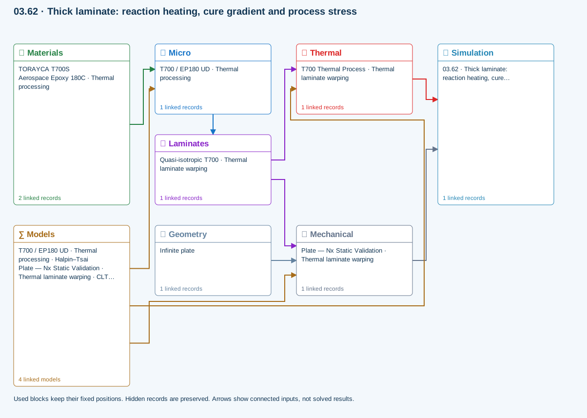
∑ Used models & submodels
Only models assigned to records used by this exercise are listed here. The full-layout option preserves the supplied starter records; no Workbench records are changed.
Halpin–Tsai · T700 / EP180 UD · Thermal processing
One compatible homogenization model per Micro recipe. Separate recipes compare models; their predictions are not blended.
∑ Theory & assumptionsCLT · Linear static with failure indices · Plate — Nx Static Validation · Thermal laminate warping
Shared laminate stiffness drives this membrane/CLT path. Failure criteria are independent comparisons, not blended models. Fatigue is a separate assessment.
∑ Theory & assumptions1D transient heat transfer · T700 Thermal Process · Thermal laminate warping
Needs linked laminate properties and a compatible process schedule. A linked cycle is not a solved temperature history.
∑ Theory & assumptionsMaximum stress · Plate — Nx Static Validation · Thermal laminate warping
Primary ply criterion for Plate — Nx Static Validation · Thermal laminate warping. Envelope comparisons are independent; criteria are not blended.
∑ Theory & assumptionsData travelling between blocks
Micro → Laminates
Predicted ply stiffness, strength, density and expansion properties.
Materials → Micro
Constituent stiffness, strength, density and thermal / moisture properties.
Mechanical → Simulation
SIMULATION selects this case and its analysis model; the case owns its applicable cycle and input references.
Laminates → Mechanical
Ply angles and thicknesses, stiffness, mass and ply properties.
Geometry → Mechanical
Part shape and dimensions, thickness or section definition, and model-specific geometric inputs. Each selected case consumes only the dimensions its model supports.
Thermal → Simulation
SIMULATION selects this case and its analysis model; the case owns its applicable cycle and input references.
Laminates → Thermal
Ply angles and thicknesses, stiffness, mass and ply properties.
Models → Micro
Applied model assignment: Halpin–Tsai. Model parameters and formulation are used by Micro.
Models → Mechanical
Applied model assignment: CLT · Linear static with failure indices. Model parameters and formulation are used by Mechanical.; Maximum stress
Models → Thermal
Applied model assignment: 1D transient heat transfer. Model parameters and formulation are used by Thermal.
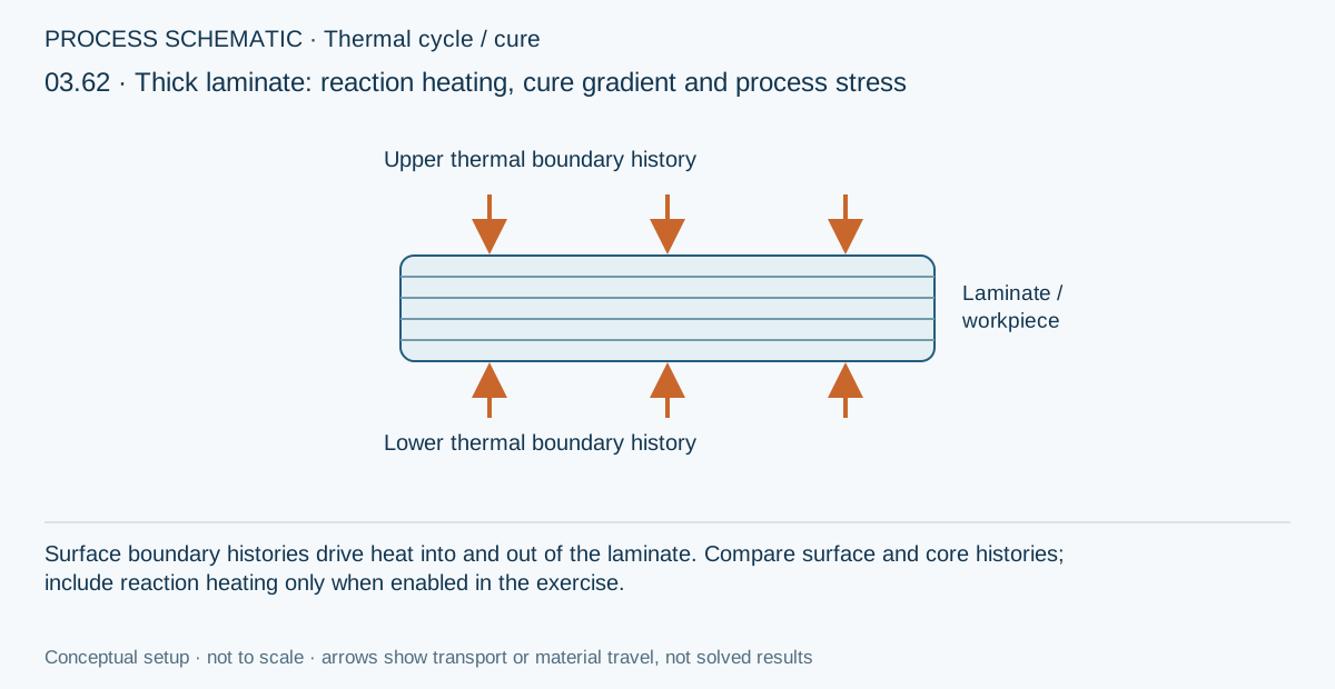
Run the 6 mm laminate through the 120°C dwell with its linked resin reaction heat.
Models: Heat transfer · Classical laminate theory · Extension–bending coupling · Thermomechanical coupling
Study scope and limitations
Teaching inputs, not qualified allowables. Sequential coupling transfers the reported thermal/moisture state to laminate mechanics; it is not simultaneous 3D multiphysics. Inspect the transferred state and reference values before interpreting stress or curvature. Free laminate CLT curvature, not fixture-constrained distortion, a full tool-release simulation or calibrated cure-shrinkage prediction.
What the study needs
| Choice | Why it matters |
|---|---|
| Material and layup | Elastic properties and fiber directions determine stiffness; strengths and fracture data are needed for the selected failure models. |
| Geometry and support | Shape, dimensions and boundary conditions determine how a component deforms and carries load. |
| Mechanical loads | Specify the forces and moments, including which components increase during progressive failure. |
| Process and environment | Temperature, moisture and material state can produce expansion, shrinkage and residual stresses. |
Define the surfaces and the material state
- Give the upper and lower surfaces independent histories when their surroundings differ.
- Choose prescribed temperature, convection or another supported thermal boundary condition.
- Define moisture exposure and the corresponding diffusion properties when studying uptake or drying.
- Provide calibrated cure or crystallization kinetics for reacting materials; use an inert material when no reaction is intended.
- A recorded pressure history is not, by itself, proof that pressure has been mechanically coupled. Check the selected structural loads.
Named response and traceability outputs
| Named result group | Contents |
|---|---|
| Transport histories | Transport metadata, time, temperature, and moisture |
| Material-state histories | Cure/crystallinity states, rates, heat sources, and shrinkage |
| Surface and ply summaries | Interpolated surfaces and final per-ply process summary |
| Process-to-structure results | Structural mapping, process-only field contributions, and process resultants |
| Double-Double recommendation | Compatibility, recommended angles, stiffness error, and selected ply angles |
| Structural summary | Cylinder summary plus plate/beam section, response, energy, buckling, and frequency results |
| Cylinder load history | Cylinder loads and resultants |
| Cylinder stress recovery | Final radial-coordinate and recovered-stress table |
Interpret before comparing. Check the final material state and residual stresses, then compare the loaded response. Missing transport or strength data must not be treated as a validated pass. Try the coupled exercise →
5.5 Resolve the thermal history before structural loading.
06.1 Manuals · read online, preview or download →
Theories / Thermal
Create independent thermal surface schedules, solve heterogeneous heat transport, evolve polymer state, and map temperature fields into laminate residual stress.
Theory map
Models, equations, figures, and cross-referencesTransient heat through thickness
Finite-volume conduction with heterogeneous plies, independent surfaces, reaction heat, and interpolated schedules.
Open heat theory →Cure and crystallization
Route thermoset cure or thermoplastic crystallization into heat generation, shrinkage, and structural mapping.
Open material-state theory →Complete reference
One continuous sequence5.6 Crystallization consolidation and interface bonding
Follow the solved thermal and pressure histories into polymer crystallinity, a local void cell and an interply bond line. Each calculation has a different state variable and a different physical meaning.
Where these models enter the workflow
The optional WB5 thermoplastic models are history-driven calculations attached to a transient thermal case. Solve the temperature history first, then evaluate crystallization at each saved thermal node, void consolidation at a selected depth, and contact and healing at a selected interface. A model must be explicitly linked to the case; a material name or an unlinked model record does not activate it.
These models currently use one-way postprocessing. Their evolving states do not change the thermal solution, layer thickness used by that solution, laminate stiffness or residual stress. In particular, the PEEK branch described here does not return latent heat or crystallization shrinkage to the solver. The separate coupled crystallization formulation in the material-state chapter describes a different execution path. Do not assume that its feedback terms are active when using the optional PEEK history model.
The workflow is: material and boundary data → transient temperature and selected pressure histories → crystallization, void or interface model → state history and interpretation. Void content measures gas in a cell; intimate contact measures touching interface area; healing describes molecular interdiffusion on that area. None of these quantities can be substituted for another.
PEEK crystallization kinetics
The parallel and series Velisaris–Seferis records represent two crystallization contributions, each advanced with a nonisothermal Nakamura clock. For branch i, let αᵢ be its relative conversion, nᵢ its Avrami exponent and Kᵢ(T) its temperature-dependent rate in inverse seconds. The accumulated clock preserves thermal history rather than recalculating conversion from the current temperature alone.
The initial clock reproduces the supplied initial conversion. A branch initially at complete conversion remains saturated until the full-melting reset. The distinction between K and the isothermal Avrami coefficient k is important: K = k1/n, so K has units s⁻¹ while k has units s⁻ⁿ. Entering k directly in the K table changes both units and kinetics.
The contribution weight w lies between zero and one. The series combination is zero when a branch with nonzero weight has zero conversion; a branch of zero weight is excluded without division by zero. X is the absolute matrix crystallinity on the basis supplied with Xmax, not the crystallinity of the fiber-filled composite. The interface reports matrix crystallinity, relative crystallinity, and the primary and secondary conversions as percentages.
Five editable temperature points define each K table. Rates are interpolated linearly, with zero endpoint values and no growth outside the specified window. The algorithm splits a saved temperature segment at each table knot and at the full-melting threshold. It then integrates the piecewise-linear interpolation exactly. At or above the melting threshold both clocks are reset to zero, allowing recrystallization on cooling. This instantaneous complete-melting rule is a modeling extension; partial melting, reorganization and melting-rate kinetics are not resolved.
Use DSC measurements from the actual polymer grade and relevant thermal histories to fit the rate tables, exponents, contribution weight and limiting crystallinity. The published parallel exponents 2.5 and 1.5 provide a literature example, but the seeded WB5 rate values, weight, limiting fraction and melting threshold are illustrative inputs rather than a fitted Seferis dataset. The series exponents also require calibration. Both records currently apply the same matrix kinetics at every thermal node; they do not assign different polymers to different layers. The formulation and implementation must be distinguished from a legacy file named crystallization.m whose coefficients describe degradation rather than crystallization.
Single cell void consolidation
The void model is a uniform periodic dry-fiber-bed reduction of the model of Simacek and colleagues. A cell contains incompressible fiber and resin together with a gas region. Transverse resin flow and the response of the fiber bed govern the change in cell thickness. It is a local representative cell, not a resolved distribution of interacting voids.
Let q be gas volume divided by the initial cell volume, φ₀ the initial void fraction, c = 1−φ₀, h₀ the initial cell thickness and Vf0 the initial fiber fraction. Constituent conservation gives the current thickness h, fiber fraction Vf and porosity φ directly from q.
Use compression-positive applied absolute pressure P, absolute gas pressure pg, resin viscosity η, permeability K, fixed void spacing L and effective bed viscosity ηb. Integrating the symmetric Darcy pressure profile across the cell gives a mean resin pressure pg−ηL²(ḣ/h)/(12K). Adding the compressive bed stress σb gives the balance below.
All pressures in this balance are in pascals, viscosities in Pa·s, permeability in m² and spacing in metres; q̇ is in s⁻¹. Applied pressure exceeding the gas and bed resistance reduces q. The reverse imbalance can produce rebound while flow remains active. This implementation derives its balance from the pressure field rather than copying the printed force and volume equations literally; it retains the mean gas-pressure term, a compression-consistent flow sign and dimensionally consistent resistance.
Temperature T is in kelvin in this expression, with a separately specified fitted offset Cη. A flow activation temperature freezes the geometry below the threshold. It is not a crystallization or cure calculation. The example carbon/PEEK coefficients and geometry require calibration before use with another tape. The bed modulus and effective bed viscosity can be zero, as in the source example.
Sealed gas conserves pV/T and cannot disappear at finite pressure. Vented gas remains at ambient pressure; evacuated gas provides no gas resistance. A closed vented or evacuated cell does not nucleate a new void on unloading. The reported equivalent radius is obtained from the gas cross-sectional area qh₀L and is a two-dimensional area descriptor, not a spherical bubble radius.
A backward-Euler update with bisection and step doubling controls the scalar integration error. Thermal knots, flow-threshold crossings and pressure events are resolved explicitly. Check constant-coefficient compaction, gas equilibrium, rebound, constituent conservation and maximum packing before interpreting a process run. Gas diffusion, capillarity, void migration, a void-size distribution and two-way thickness or stiffness feedback are outside this reduction.
Intimate contact under pressure
Intimate contact is the fraction of an interface whose opposing surfaces touch closely enough for molecular bonding to become possible. The WB5 contact record uses a lumped asperity squeeze-flow law. It does not resolve a fractal hierarchy of individual asperities. Pressure and effective contact-flow viscosity determine an accumulated exposure J, and a roughness coefficient Rc converts that exposure into contact fraction Dc.
J is dimensionless when pressure is in pascals, viscosity in Pa·s and time in seconds. The fifth-power initial term treats an existing contact fraction D₀ as equivalent prior exposure. It deliberately differs from adding D₀ to the zero-state fifth-root solution, which would not preserve the same constitutive state during continued loading. New contact is monotonic; reopening and contact damage are not included.
The contact viscosity uses ηc = A exp[B/(T+C)], evaluated only above the contact activation temperature. The illustrative fit A = 132.95 Pa·s, B = 2969 K and C = −273.15 K reproduces the legacy Celsius-denominator expression while T is supplied in kelvin. This empirical law must not be mistaken for an activation-energy Arrhenius law. Contact-flow viscosity is a separate parameterization from the viscosity used by the void Darcy-flow calculation.
For contact, gauge pressure is already net compression. Absolute pressure is converted by subtracting ambient pressure once, and negative net compression is clipped to zero. Global pressure excludes roller additions; an upper or lower total includes the global profile and the selected face contribution once. The two opposing pressures are not added. Unloading stops new pressure-driven contact but does not remove contact already formed.
Healing and age dependent coupled bonding
After surfaces touch, compatible thermoplastic chains need time at a sufficiently high temperature to interdiffuse across the interface. Healing therefore depends on both thermal history and the time at which each portion of the interface first made contact. A fully hot interface with no contact cannot develop a bond in this model.
The exposure integral advances only above the healing activation temperature. Welding time is in seconds, temperatures in kelvin, activation energy in J/mol and R = 8.314462618 J/(mol·K). The AS4/PEEK example uses 0.11 s at 400°C, activation energy 57300 J/mol and a 338°C activation threshold. These are example inputs, not universal values for all PEEK tapes or polymer pairs.
A new contact patch is born at time τ and begins with zero healing. The dimensionless h₀ in this section is the initial healing of the area already in contact, not the cell thickness h₀ used in the void model. Keeping these states separate prevents a late-forming patch from receiving the thermal exposure that occurred before contact.
The area integral follows Butler-type contact-age coupling with nonisothermal healing. It is not approximated by multiplying the final contact fraction by the healing potential of an interface assumed to touch from the start. The reported healing potential is useful for separating thermal opportunity from contact delay, but coupled bonding is the quantity that includes both histories. A strength is reported only when a fully healed strength is supplied; the scaling is not a qualified design allowable.
The numerical method integrates exposure with midpoint step doubling, limits the new contact area and healing exposure per step, and assigns patch birth exposures using two-point quadrature in contact area. Mature patches are accumulated as fully bonded area. Refine the maximum step, contact increment and tolerance together when checking convergence. Cooling pauses the active mechanisms, while reheating resumes their accumulated histories. Healing may continue after unloading if the interface remains hot and in contact, as assumed here. Debonding, degradation, crystallization-dependent mobility, incompatible polymers and feedback to conductivity or mechanical properties are excluded.
Model selection and verification
Use the thermal case's PEEK crystallization model link for either crystallization record, the Void consolidation model link for the cell calculation, and the contact-only or coupled-bonding links for the interface calculation. The coupled model references its contact record. If both interface links are populated, they must identify the same contact model so depth, pressure and integration assumptions cannot diverge.
Void and bond histories use a selected normalized depth, with zero at the lower surface and one at the upper surface. They are single-depth histories, not measured or predicted distributions through the complete thickness. Crystallization instead follows each saved thermal node. For a moving process with positive constant speed, distance follows x = vt; this is a time-to-position mapping, not a new spatial transport solve.
First refine the saved thermal output so heating peaks, cooling intervals and roller events are adequately resolved. Then refine each postprocessor's internal integration. An accurate integration of interpolated temperature cannot recover a peak that was never saved. Use isothermal crystallization, fifth-root contact, quarter-power healing and a delayed-contact comparison as limiting checks. Record the model IDs, coefficients, pressure convention, depth, numerical settings and parameter sources with the resulting histories. Experimental validation requires DSC, rheology, void measurements or bond tests appropriate to the quantity being predicted.
References
- Velisaris, C. N. and Seferis, J. C. (1986). Crystallization kinetics of polyetheretherketone (PEEK) matrices. Polymer Engineering and Science, 26, 1574–1581. doi:10.1002/pen.760262208.
- Nakamura and colleagues (1972). Some aspects of nonisothermal crystallization of polymers I. Journal of Applied Polymer Science, 16, 1077–1091. doi:10.1002/app.1972.070160503.
- Kelly, C., Hay, J., Turner, R. and Jenkins, M. (2020). The effect of a secondary process on the analysis of isothermal crystallisation kinetics by differential scanning calorimetry. Polymers, 12, 19. doi:10.3390/polym12010019. Used for the branch-combination relations, not PEEK calibration.
- Simacek, P., Advani, S. G., Gruber, M. and Jensen, B. (2013). A non-local void filling model to describe its dynamics during processing thermoplastic composites. Composites Part A, 46, 154–165. doi:10.1016/j.compositesa.2012.10.015.
- Tierney, J. and Gillespie, J. W. (2006). Modeling of in situ strength development for the thermoplastic composite tow placement process. Journal of Composite Materials, 40, 1487–1506. doi:10.1177/0021998306060162.
- Yang, F. and Pitchumani, R. (2002). Healing of thermoplastic polymers at an interface under nonisothermal conditions. Macromolecules. doi:10.1021/ma010858o.
- Butler, C. A., McCullough, R. L., Pitchumani, R. and Gillespie, J. W. (1998). An analysis of mechanisms governing fusion bonding of thermoplastic composites. Journal of Thermoplastic Composite Materials. doi:10.1177/089270579801100404.
5.7 Epoxy viscosity and cure
Open the matrix material, follow its Cure kinetics model, then select Resin viscosity model. Choose Castro–Macosko epoxy viscosity, edit its inputs, or choose None to disconnect it. Existing epoxy cure records gain this new link once; existing None and calibrated choices are retained.
The same local cure conversion drives two paths: temperature + cure → viscosity → resin flow; and cure → CHILE resin modulus → micromechanics → ply and laminate stiffness.
| Input | Example | Meaning |
|---|---|---|
| Reference uncured viscosity | 1 Pa·s | Viscosity at zero conversion and the reference temperature. Illustrative, not a product calibration. |
| Viscosity reference temperature | 80 °C | Temperature at which the reference uncured viscosity is specified. |
| Viscosity activation energy | 45 kJ/mol | Arrhenius temperature dependence; illustrative coefficient. |
| Viscosity gel conversion | 0.55 fraction | Flow stops at this conversion. Match the resin kinetics and CHILE gel inputs when fitting the material. |
| Viscosity cure coefficient C1 | 2 — | Positive fitted exponent constant. |
| Viscosity cure coefficient C2 | 0 — | Nonnegative fitted conversion coefficient. |
| Viscosity reporting ceiling | 1000000000000 Pa·s | Numerical plotting ceiling; the gelled resin is flow-inactive, not a flowing liquid at this viscosity. |
Equation and limits
η = ηref exp[(Eη/R)(1/T − 1/Tref)] [αg/(αg − α)]^(C1 + C2 α). Temperatures are kelvin; conversion is a fraction. Flow ceases at gel. The plotted viscosity ceiling is a numerical reporting value, not post-gel liquid behavior.
Defaults are illustrative screening inputs, not measurements for a branded resin. Match the viscosity, kinetics and modulus gel parameters during calibration. This formulation does not include shear thinning, vitrification or degradation. CHILE supplies elastic stiffness independently; viscosity does not determine modulus. Void reduction remains one-way postprocessing and does not alter the structural fiber fraction or thickness.
IACMI/Purdue report: Castro–Macosko viscosity, p.9After Run, Thermal → Solved thermal field offers Epoxy viscosity, Epoxy pre-gel flow active, resin modulus and lamina E1/E2/G12. Refine the thermal output interval to resolve rapid cure. Roller and gel-crossing events are retained by the flow integrations.
5.8 Thermoplastic prepreg processing
Prepreg 03 and 05 use eight 0.125 mm T700/PEEK plies, [0/90]2s. Run these examples to see melt flow, voids, intimate contact and healing across all seven interfaces. Prepreg 01, 02 and 04 use thermoset epoxy with cure and CHILE stiffness; thermoplastic healing is disconnected.
Open the PEEK material to edit its Resin viscosity model and Viscoelastic modulus model. In the thermal case, Initial conditions selects Void consolidation, Intimate contact, Interface bonding and Material model sampling. Roller force produces the shared pressure through all plies.
Thermal results offer melt viscosity, flow-active state, SLS matrix modulus, SLS unit-step relaxation and lamina E1/E2/G12. Select interfaces or plies in the material-state plots to inspect bonding and voids.
Thermoplastic Arrhenius melt viscosity
| Model family | Thermoplastic Arrhenius melt viscosity model |
|---|---|
| Melt viscosity prefactor | 0.016384 Pa·s |
| Melt viscosity coefficient | 6403 K |
| Melt viscosity offset | 30 K |
| Melt flow activation temperature | 343 °C |
| Viscosity reporting ceiling | 1000000000000 Pa·s |
| Formulation | eta = A exp[B/(T[K]+C)]. Flow pauses at/below activation temperature; solid-state ceiling is reporting only. |
| Parameter basis | PEEK example flow law retained from the existing void-cell example. Using it for interface squeeze flow is a teaching assumption requiring surface-specific calibration. |
| Source | https://doi.org/10.1016/j.compositesa.2012.10.015 |
| Assumptions | Zero-shear temperature law. No cure, shear thinning, degradation or crystallinity feedback. Melt viscosity is independent of the SLS dashpot viscosity. |
Thermoplastic standard linear solid
| Model family | Thermoplastic standard linear solid model |
|---|---|
| Instantaneous resin modulus | 3.6 GPa |
| Equilibrium resin modulus | 0.0036 GPa |
| Reference relaxation time | 10 s |
| Relaxation reference temperature | 143 °C |
| Relaxation activation energy | 100 kJ/mol |
| Modulus observation time | 1 s |
| Formulation | E(t,T)=Einf+(E0-Einf) exp[-t/tau(T)]; tau(T)=tauRef exp[Ea/R(1/T-1/Tref)]. |
| Parameter basis | Illustrative PEEK-like relaxation spectrum; fit E0, Einf, tau and temperature shift to measured DMA/relaxation data. Not a grade calibration. |
| Assumptions | Thermorheologically simple SLS with constant branch springs and Poisson ratio. Nonzero equilibrium modulus is a solid approximation, not a molten-fluid law. Micro/CLT use observation-time modulus; thermal stresses are equivalent-elastic, not a hereditary laminate stress solve. Unit-step relaxation is also reported. |
| Source | https://doc.comsol.com/6.3/doc/com.comsol.help.sme/sme_ug_theory.06.029.html |
SLS is an equilibrium spring in parallel with one Maxwell branch. It predicts E(t,T) = Einf + (E0 − Einf) exp(−t/τ(T)). The explicit observation time sets the stiffness used by micromechanics and equivalent-elastic thermal CLT. It is independent of the thermal output interval. The separate unit-step relaxation plot integrates reduced time along the thermal history.
This release does not solve full hereditary laminate stresses, crystallization feedback, melt latent heat or degradation. The SLS equilibrium spring approximates a soft solid; melt-flow viscosity is a separate law. All new material coefficients are editable teaching inputs, not certified PEEK data.
SLS and temperature-shift formulation5.9 PEEK crystallization · Velisaris–Seferis
Two model records track primary and secondary crystallization. Parallel is a weighted sum; series is a harmonic combination. Both follow the temperature histories at thermal nodes or use ply-average temperatures, according to the thermal case sampling setting.
Set up
- Open Models → Thermoplastic Crystallization. Copy either PEEK · Velisaris–Seferis parallel or series.
- Set the two exponents, contribution weight, initial conversions, maximum matrix crystallinity and five temperature/rate points. The supplied values are illustrative, not a validated PEEK-grade calibration.
- In Thermal → Initial conditions → Optional PEEK crystallization, select the model. This explicit case assignment applies one matrix formulation across all sampled nodes or plies. A material’s older Crystallization model link alone does not activate this case calculation.
- Run a transient thermal cycle. The existing moving-process velocity maps residence time to position.
- In the 2D thermal field dropdown choose PEEK matrix crystallinity, Relative crystallinity, Primary crystallization conversion or Secondary crystallization conversion. Move the cursor to inspect time and thickness sections. Expand calibration and assumptions for model provenance.
What the results mean
Primary and secondary conversions are dimensionless process progress, each from 0–100%. Relative crystallinity combines those processes. Matrix crystallinity is that combined value multiplied by the specified limiting matrix crystalline fraction; it is not the crystalline fraction of the entire fiber/resin composite.
Equations and temperature history
Each branch has qᵢ = qᵢ₀ + ∫Kᵢ(T)dt and αᵢ = 1 − exp(−qᵢⁿⁱ). Initial clocks reproduce the supplied initial conversions. At constant temperature, the usual Avrami coefficient is kᵢ = Kᵢⁿⁱ. Enter K in 1/s; do not enter k in s⁻ⁿ.
Parallel: α = wα₁ + (1−w)α₂. Series: α = 1/[w/α₁ + (1−w)/α₂]. With a positive weight and zero conversion in either branch, the series result is zero. Series does not impose a hard delayed start for the secondary clock. Matrix crystallinity is X = Xmax α.
The nonisothermal implementation uses Nakamura accumulation. K is linearly interpolated between the editable table points and is zero outside that window. Thermal segments split at every rate-table knot, so integration is exact for the saved piecewise-linear temperature history. Refine thermal output spacing to capture short heating pulses; plot smoothing cannot recover an unsaved peak.
Inputs
| Control | Function |
|---|---|
| Model family (model) | Parallel weighted sum or series harmonic combination of two Avrami conversions. |
| Primary Avrami exponent (—) | Published parallel PEEK fit exponent. Refit for the series variant or another material grade. |
| Secondary Avrami exponent (—) | Published parallel PEEK fit exponent; not a universal PEEK constant. |
| Primary contribution (%) | Illustrative fixed weight. Secondary weight is 100% minus this value. Calibrate both mechanisms together. |
| Initial primary conversion (%) | Initial relative conversion of the primary process, not absolute matrix crystallinity. |
| Initial secondary conversion (%) | Initial relative conversion of the secondary process. Initial states are mapped to equivalent accumulated kinetic clocks. |
| Maximum matrix crystallinity (%) | Illustrative limiting crystalline fraction of the matrix, not composite fiber-plus-resin mass. Use one consistent mass or volume basis from calibration. |
| Full melting temperature (°C) | Simplified instantaneous full-melt reset at/above this temperature. No partial melting kinetics. This is a CDS extension, not the original crystallization equation. |
| Kinetics temperature 1 (°C) | Illustrative temperature grid. Strictly increasing; outside the table growth pauses. Endpoint rates must be zero. |
| Primary K 1 (1/s) | Illustrative Nakamura rate K = k^(1/n). Enter fitted primary rates; interpolation is linear in K, with time in seconds. |
| Secondary K 1 (1/s) | Illustrative secondary Nakamura rate. These table rates are not published Seferis coefficients. |
| Kinetics temperature 2 (°C) | Illustrative temperature grid. Strictly increasing; outside the table growth pauses. Endpoint rates must be zero. |
| Primary K 2 (1/s) | Illustrative Nakamura rate K = k^(1/n). Enter fitted primary rates; interpolation is linear in K, with time in seconds. |
| Secondary K 2 (1/s) | Illustrative secondary Nakamura rate. These table rates are not published Seferis coefficients. |
| Kinetics temperature 3 (°C) | Illustrative temperature grid. Strictly increasing; outside the table growth pauses. Endpoint rates must be zero. |
| Primary K 3 (1/s) | Illustrative Nakamura rate K = k^(1/n). Enter fitted primary rates; interpolation is linear in K, with time in seconds. |
| Secondary K 3 (1/s) | Illustrative secondary Nakamura rate. These table rates are not published Seferis coefficients. |
| Kinetics temperature 4 (°C) | Illustrative temperature grid. Strictly increasing; outside the table growth pauses. Endpoint rates must be zero. |
| Primary K 4 (1/s) | Illustrative Nakamura rate K = k^(1/n). Enter fitted primary rates; interpolation is linear in K, with time in seconds. |
| Secondary K 4 (1/s) | Illustrative secondary Nakamura rate. These table rates are not published Seferis coefficients. |
| Kinetics temperature 5 (°C) | Illustrative temperature grid. Strictly increasing; outside the table growth pauses. Endpoint rates must be zero. |
| Primary K 5 (1/s) | Illustrative Nakamura rate K = k^(1/n). Enter fitted primary rates; interpolation is linear in K, with time in seconds. |
| Secondary K 5 (1/s) | Illustrative secondary Nakamura rate. These table rates are not published Seferis coefficients. |
| Source (source) | Velisaris & Seferis (1986), PEEK two-process crystallization. |
| Parameter basis (text) | Source-grounded formulation; this seed is not a validated PEEK material calibration. |
Calibration and scope
The original parallel PEEK exponents are 2.5 and 1.5. The seeded rate table, weight, maximum fraction and melting temperature are illustrative CDS inputs, not original Seferis fitted coefficients. The series record requires a separate fit. Calibrate against DSC data for the actual polymer grade, reinforcement and cooling-rate range.
This version postprocesses the solved temperature field. It does not feed latent heat, crystallization shrinkage or evolving stiffness into the solver, or modify the separate intimate-contact/healing calculation. It assumes one PEEK matrix throughout the thermal section. Pressure dependence, heterogeneous polymer assignments, high-rate correction and partial melting are outside this version.
Full melting resets both clocks instantaneously at the editable threshold; cooling permits renewed crystallization. This reset is a simplified CDS extension, not a fitted melting model. Below the rate window, crystallinity is retained.
Sources
- Velisaris & Seferis (1986): PEEK crystallization kinetics
- Kelly et al. (2020): parallel and series formulations, equations 6–7
- Pérez-Martín et al. (2022): dual-process and Nakamura nonisothermal formulation; PEKK study, not PEEK parameter calibration
Node, interface and ply sampling
In Thermal → Initial conditions → Material model sampling, choose All thermal nodes or Interfaces and ply averages, then rerun. All thermal nodes evaluates each linked void, interface and PEEK model at every thermal node. Reduced sampling evaluates contact/healing only at internal ply boundaries and evaluates voids/PEEK using each ply's thickness-averaged temperature.
An eight-ply laminate has seven internal interfaces and eight ply histories. The outer surfaces are excluded from the interface count. Ply numbering runs from the lower face to the upper face. The linked model coefficients, initial states and pressure source apply at every sampled location.
Select a material output in the temperature dropdown, then choose All interfaces or All ply results. Each location has a separate trace, a visibility checkbox and a value at the slicer time cursor. Moving runs support distance; Slice CSV exports all traces. With node calculations, the slicer can also show all thermal nodes. Cursor output retains the existing detailed plot; reduced PEEK results use the ply slicer and its time cursor.
Reduced mode averages temperature before running the nonlinear bulk model. In node mode, the ply slicer averages already calculated results, while interface traces interpolate node results. These operations can differ. Compare the two modes when temperature varies strongly across a ply. The thermal mesh, cure/reaction model and saved thermal output interval are unchanged.
Model defaults preserves older studies: void and interface models use their chosen depth; PEEK uses thermal nodes. Older saved runs need a new run with a sampling mode selected to produce material slices. PEEK rate coefficients remain illustrative and require calibration.
5.10 Intimate contact, healing and coupled bonding
Epoxy contact can use cure-dependent resin viscosity. Flow stops at gel. The thermoplastic healing model must be disconnected for this epoxy calculation.
These two model records describe a thermoplastic bond line. Intimate contact predicts how much of the nominal surface actually touches; healing describes polymer interdiffusion across contact; coupled bonding accounts for the different times at which each area first touches.
Set up and run
- In Models → Interface Bonding, copy the Intimate Contact Model example. Set its interface depth, pressure source, surface coefficient and viscosity law for the tape.
- For healing and bonding, copy Interface Healing and Coupled Bonding Model and select the contact record inside it. Set welding-time coefficients and initial healing. Fully healed bond strength is optional.
- In the transient Thermal case → Initial conditions → Optional interface bonding, select the contact model for contact-only results, or select the bonding model for both calculations. You do not need both case links. If both are set they must reference the same contact model.
- Run the existing temperature and pressure schedule. Global pressure excludes rollers; Total uses one shared global-plus-roller pressure on both faces. Opposing roller pressures are not added. Time and length schedules use the existing travel-velocity conversion.
- In the 2D thermal dropdown select Intimate contact and bonding profile. Compare all three percentages or choose temperature, pressure, viscosity, welding time or scaled strength. Moving runs offer Time/Distance. Bonding CSV exports every saved quantity.
Meaning of the curves
Contact is the percentage of nominal area touching. Healing potential assumes contact existed from the beginning and is an upper reference, not the actual bond. Coupled bonding is the area-weighted healing of patches created at their own contact times. It cannot exceed contact. A 100% bonding index is model saturation, not a structural qualification or measured strength.
Equations
Contact exposure J = ∫ Pnet/η dt. The lumped asperity model uses Dcontact = min(1, [D0⁵ + Rc⁵ J]¹ᐟ⁵). For zero initial contact this is the Mantell–Springer form used by Tierney and Gillespie. Nonzero initial contact uses an equivalent prior exposure; it deliberately differs from adding D0 after the fifth root in the empirical contact formulation code.
Viscosity is η = A exp(B/(T[K]+C)). The supplied legacy contact fit has A=132.95 Pa·s, B=2969 K and C=−273.15 K, reproducing its empirical Celsius denominator. Do not reinterpret it as a kelvin Arrhenius fit. Use calibrated effective surface-flow viscosity.
Yang–Pitchumani healing uses H(t)=∫dt/tw(T), with tw=tw_ref exp(Ea/R [1/T−1/Tref]) and kelvin temperatures. A patch born at τ heals by min(1, [H(t)−H(τ)]¹ᐟ⁴). Existing initial contact can start with a specified healing level. The Butler coupling is Db(t)=D0 Dh_initial(t)+∫Dh(τ,t)dDcontact(τ).
The AS4/PEEK example welding time is 0.11 s at 400°C, activation energy 57.3 kJ/mol, and activation threshold 338°C. Coefficients for other materials must be measured or otherwise justified. Surface roughness and viscosity are independent of the void model’s permeability and pore-flow viscosity.
Controls
Intimate Contact Model
| Input | Example | Function |
|---|---|---|
| Model family | Intimate Contact Model model | Editable model coefficient; see equations above. |
| Initial intimate contact | 0 % | Initial fraction of interface already touching. Prior exposure is initialized as D0^5, preserving continuity under subsequent flow. |
| Surface roughness coefficient | 0.29 — | Lumped asperity coefficient Rc. AS4/PEEK example reported by Tierney and Gillespie; calibrate to tape surfaces. |
| Contact viscosity prefactor | 132.95 Pa·s | Empirical contact fit: eta=A exp(B/(T[K]+C)). Effective surface-flow viscosity, not necessarily neat resin viscosity. |
| Contact viscosity coefficient | 2969 K | Editable model coefficient; see equations above. |
| Contact viscosity offset | -273.15 K | The legacy empirical fit uses Celsius in the denominator. Offset −273.15 K reproduces it. This is separate from the kelvin Arrhenius healing law. |
| Contact activation temperature | 338 °C | AS4/PEEK example melt threshold. Contact growth stops at/below this value; existing contact persists. |
| Interface depth | 0.5 fraction | 0=lower face, 1=upper face. Set to the intended ply bond line. One selected interface per case; not an automatic distribution. |
| Interface pressure source | Total type | Total is the shared through-thickness pressure: global plus the largest active roller contribution. Opposing nip pressures are not added. Global excludes rollers. |
| Interface pressure convention | Gauge type | Gauge is net compression; absolute subtracts ambient once. Negative net pressure creates no new contact. |
| Interface ambient pressure | 0.1 MPa absolute | Editable model coefficient; see equations above. |
| Maximum bonding step | 1 s | Internal steps also resolve schedule events, temperature thresholds and contact/healing increments. |
| Maximum contact increment | 0.5 % | Maximum area gained per internal step. Reduce to check coupled bonding convergence. |
| Bonding integration tolerance | 0.000001 fraction | Controls midpoint step-doubling for pressure/viscosity and reciprocal welding-time integrals. |
| Parameter basis | AS4/PEEK example; Rc from Tierney–Gillespie, viscosity from empirical contact formulation; calibrate for the actual tape text | Editable model coefficient; see equations above. |
Interface Healing and Coupled Bonding Model
| Input | Example | Function |
|---|---|---|
| Model family | Interface Healing and Coupled Bonding Model model | Editable model coefficient; see equations above. |
| Intimate contact model | MOD-CONTACT-001 ref | Required linked contact model supplies surface flow, interface depth, pressure convention and integration settings. |
| Initial healing of existing contact | 0 % | Applies only to area already in contact initially. New areas start unhealed. |
| Reference welding time | 0.11 s | AS4/PEEK example: full-healing time at the reference temperature, reported in Tierney–Gillespie from Yang–Pitchumani. |
| Healing activation energy | 57300 J/mol | tw(T)=tw_ref exp(Ea/R [1/T−1/Tref]); both temperatures in kelvin. |
| Healing reference temperature | 400 °C | Editable model coefficient; see equations above. |
| Healing activation temperature | 338 °C | Healing pauses at/below this example PEEK melt threshold. Retains exposure on cooling and reheating; no crystallization kinetics. |
| Fully healed bond strength | Optional MPa | Optional calibrated strength. Blank reports dimensionless bonding only; no strength is invented. |
| Parameter basis | AS4/PEEK example; compatible thermoplastic surfaces only. Includes contact delay in healing; calibrate before strength prediction. text | Editable model coefficient; see equations above. |
Scope and convergence
This version postprocesses one selected interface from the solved temperature history. Net compressive pressure drives new contact. Established contact is retained on unloading, and healing may continue while hot even after a roller leaves. Cooling below a threshold pauses that mechanism; reheating resumes it. The model does not predict reopening, damage, degradation, crystallization, thermoset chemical bonding, or mismatched polymer compatibility. It does not change thermal conductivity, laminate thickness or mechanical properties.
Integration resolves schedule knots, roller pressure events, activation crossings and bounded contact/healing increments. Reduce maximum step, maximum contact increment and tolerance to check numerical convergence; refine saved thermal output for rapid heating. The simple lumped asperity law is implemented here, not the full Yang–Pitchumani fractal contact model.
References
- Tierney & Gillespie (2006): in-situ tow-placement strength development
- Yang & Pitchumani (2002): nonisothermal healing
- Butler, McCullough, Pitchumani & Gillespie (1998): coupled fusion bonding
- Bastien & Gillespie (1991): earlier nonisothermal healing work
Node, interface and ply sampling
In Thermal → Initial conditions → Material model sampling, choose All thermal nodes or Interfaces and ply averages, then rerun. All thermal nodes evaluates each linked void, interface and PEEK model at every thermal node. Reduced sampling evaluates contact/healing only at internal ply boundaries and evaluates voids/PEEK using each ply's thickness-averaged temperature.
An eight-ply laminate has seven internal interfaces and eight ply histories. The outer surfaces are excluded from the interface count. Ply numbering runs from the lower face to the upper face. The linked model coefficients, initial states and pressure source apply at every sampled location.
Select a material output in the temperature dropdown, then choose All interfaces or All ply results. Each location has a separate trace, a visibility checkbox and a value at the slicer time cursor. Moving runs support distance; Slice CSV exports all traces. With node calculations, the slicer can also show all thermal nodes. Cursor output retains the existing detailed plot; reduced PEEK results use the ply slicer and its time cursor.
Reduced mode averages temperature before running the nonlinear bulk model. In node mode, the ply slicer averages already calculated results, while interface traces interpolate node results. These operations can differ. Compare the two modes when temperature varies strongly across a ply. The thermal mesh, cure/reaction model and saved thermal output interval are unchanged.
Model defaults preserves older studies: void and interface models use their chosen depth; PEEK uses thermal nodes. Older saved runs need a new run with a sampling mode selected to produce material slices. PEEK rate coefficients remain illustrative and require calibration.
5.11 Laser heating for moving prepreg and AFP
ATP development preview: this section documents the current implementation, not an announced major release. Check release status and confirmed scope before relying on availability.
Use the Upper boundary toolbar → Laser / AFP. Choose Overhead for a beam normal to a moving workpiece, or AFP nip for separate incoming tape and substrate fields coupled at an upper roller. The preheater starts disabled. Laser cases currently support one roller; this prevents silently omitting other tooling shadows.
Inputs and geometry
Power is total optical power at the defined aperture. Rectangle and ellipse spots are uniform; Gaussian uses the half-dimensions as 1/e² radii, truncated at the rectangular aperture and normalized to total power. A custom rectangular grid defines relative intensity. Dimensions are measured in the plane normal to the collimated beam. Tilt is measured from vertical; target position, target height and lateral offset locate the beam. Stand-off translates its origin without changing its collimated spot.
The AFP tape approaches tangentially, wraps the selected roller and joins the substrate at the predicted nip entry. Select an Incoming tape supply to use an independent material and its width, thickness, fiber/void fractions and optical defaults. With None selected, the tape uses a selected ply of the case laminate and separately specified dimensions. Each face has its own transient temperature. After contact, the two slabs exchange heat through the specified conductance, while the roller acts on the tape’s outer face. Substrate and tape travel at the web speed. The optional preheater is a two-sided film-temperature zone measured upstream along the tape path.
Roller precycling and optical reuse
In roller thermal settings, select Precycle · N revolutions. One cycle is one full turn at the selected RPM or no-slip web speed. Warm-up lasts N / RPM minutes, then the normal process continues from the complete radial and circumferential temperature field. The roller plot marks this handoff. Zero cycles is a cold start; a fixed N is not a steady-state convergence test. The existing continuous-feed approximation uses a web contact temperature iterated with the process solution.
Laser and IR now reuse independent in-memory unit-power ray solutions. Changing one source geometry or optical properties recalculates that source. Shared tape/roller/substrate geometry changes recalculate both. Power changes scale the cached distributions; temperature and warm-up changes do not retrace rays. Caches can be rebuilt after a worker restart or eviction.
Incoming tape preheat boundaries
Laser / AFP → Incoming tape → Tape preheat offers Off, Simple (both faces), or a Two-face boundary table. Bonding face points toward the substrate; Roller face contacts the tool. Start and End are millimetres upstream along the angled tape, with Start greater than End. Step holds the entered start temperature; Ramp moves from start to end temperature in the travel direction. Nonoverlapping zones on each face support convection, tool contact, IR flux, convection plus IR, prescribed temperature or insulation. IR flux is incident radiant W/m² multiplied by the entered efficiency. Uncovered distances use the air settings.
The two-face table replaces the simple preheater. Longer zones extend the tape inlet and preheat exposure independently of substrate residence. Each face retains its temperature through the wrap and nip: roller contact replaces the roller-face boundary on the wrap, then tape/substrate contact replaces the bonding-face boundary at deposition. Prescribed tape temperatures use an ideal thermostat with its supplied energy included in the balance. Separate laser and finite IR emitter heating remain additive; avoid representing one physical heater twice. Enable the coupled tape / laser / IR model and set laser power to zero for preheat-only comparisons.
Incoming tape results show both face temperatures, mean tape temperature and substrate bonding-face temperature against tape distance or elapsed tape time. Wrap and nip markers locate the change to contact. The section slider shows all nine solved tape temperature nodes through thickness. Programmed preheat plots show environment temperatures or absorbed zone IR until contact takes precedence; these are boundary inputs, not net heat flux. Tape CSV exports the histories and profiles. Existing saved runs need rerunning for section data. Live Process shows separate colored face zones along the actual angled tape.
Tape supply specifications
Materials → Tape supplies stores editable supply specifications. The seeded CF/PEEK tape is Example data, not vendor data. Record a vendor baseline only after entering the supplier specification and identifying its source and revision. Ordinary edits preserve that baseline and show Modified from vendor data with a field-by-field comparison. Restore baseline values stages the original values; Apply specification saves them. The comparison covers the listed supply fields, not changes within linked material or model records.
Upper → Laser / AFP → Incoming tape selects the supply. Its material is independent of the substrate laminate. Enable the case dimensions / optics override to make a local change without editing the shared supply. Run results retain the supply status and changed-field names used for that run. Initial crystallinity is retained as supply metadata; incoming tape bulk crystallization is not currently solved.
Live Process
Open Live Process beside the boundary plot. Configured AFP nip settings show the incoming tape wrapping onto the roller and deposited tape, including when heating is disabled (geometry preview only). Enabled laser settings add an angled schematic head, the true-size aperture and sampled first-hit beam guides. Spot overlay shows the nominal projected footprint clipped to finite tape, substrate and roller facets; edge shadows use the facet resolution. It is a geometric preview, not an absorbed-intensity map. Focus nip fits the laser and roller together. The head housing is schematic; aperture dimensions, placement and angle follow the model. The optional orange preheat band follows the configured upstream distances along the tape. Select an element to inspect its settings and fit the view; scroll to zoom or switch to 3D and drag to rotate. Laser / AFP opens the same case settings directly in this view. Preheat is off by default; its temperature, film coefficient and upstream limits are editable. Only the part of the preheater after the modeled tape inlet is calculated. Enable Absorbed flux for a current-input optical calculation in Live Process. The color map resolves Gaussian intensity across the surface; side view shows the width-average flux. The displayed composite efficiency is (tape absorbed W + substrate absorbed W) / emitted W. The optical calculation runs separately so rotating and zooming remain responsive. Run the thermal model for temperatures.
Optical model
Finite-width facets intercept directional rays and resolve shadowing by the roller and tape. Each hit absorbs energy according to an editable spectral normal absorptance and an effective Schlick grazing correction. Reflected power is split between specular rays and a diffuse exchange model. Reciprocal, visibility-tested centroid view factors distribute the diffuse part. A common normalization limits row sums while retaining reciprocity; refine the facet resolution for close surfaces. Unabsorbed rays and unfinished reflection tails are reported separately. Optical conservation checks incident = absorbed + escaped + unresolved power.
Wavelength selects/interpolates supplied absorption data. No extrapolation is performed. The example 980 nm coefficients are illustrative inputs, not measurements from the cited papers. This effective model does not reproduce the published anisotropic micro-half-cylinder BRDF. Changing wavelength without appropriate optical data is not a calibrated prediction.
Absorbed power and depth heating
The Gaussian aperture distribution is proportional to exp[−2(u²/a² + v²/b²)], with a and b equal to the specified half-sizes. Its discrete ray powers are normalized to total optical power. Ray intersections account for angle, projected surface area and shadows; absorption uses the wavelength-dependent material inputs. Live Process shows absorbed flux in W/m², including the cross-width distribution of direct and specular rays. The diffuse contribution is averaged across each facet. The thermal solution is still a width-average through-thickness model, not a three-dimensional temperature field.
Surface + conduction applies net absorbed power at the illuminated face. Optional Depth profile + conduction distributes that same power using a normalized exponential: Q(z) = q_abs exp(−z/δ) / [δ (1 − exp(−H/δ))]. Q is W/m³; z is normal depth from the illuminated face; H is body thickness; δ is the effective absorption depth. Cell-integrated power sums exactly to q_abs, so efficiency is not applied again. This is a conditional deposition profile for measured net absorptance, not a transmission model through a thin tape, resin/fiber microstructure or ply stack. The example 0.02 mm depths are illustrative and must be replaced with material data at the selected wavelength. Tape and substrate can use different depths. The roller retains surface absorption.
The current beam is collimated. Changing stand-off moves its aperture and can change visibility; it does not invent beam divergence or inverse-square spreading. Spot dimensions define the aperture and remain constant along the beam.
Optional reflections and IR emitter
Upper → Laser / AFP → Energy distribution lets you turn reflected exchange off. Direct beam size, angle and first-hit shadows remain active. With reflections off, unabsorbed power escapes. With reflections on, the laser uses mixed specular/diffuse exchange; IR uses diffuse reflection.
Optional IR emitter adds a rectangular diffuse radiant face with width, length, centre, height, lateral offset and tilt. Emitted flux is W/m² of emitter area, so radiant power equals flux × area. It is not electrical lamp power. Separate broadband tape, substrate and roller absorptances are editable examples. A deterministic cosine-weighted hemisphere integration calculates finite-source interception with tape/roller shadowing, equivalent to the visible cos θ₁ cos θ₂ / (π R²) view-factor integral. Standard uses 16,384 rays; Fine uses 65,536. Compare resolutions for small targets. IR always deposits at the incident surface, including the opposite face of the incoming tape when illuminated. The model does not include temperature-dependent thermal re-emission or an emitter temperature solve. Existing Convection + IR flux is additive; set it to zero if this emitter already represents that heater.
Live Process → Absorbed flux → Energy distribution separates each source’s tape/substrate/roller interception fractions and absorbed watts. The IR fractions are source view factors; laser fractions are directional interception. Geometric surface-exchange factors and unit-power distributions are cached in memory. Power changes scale the cached distributions. Temperature, contact conductance and preheat changes do not retrace optics. Spot, position, angle, optical data, resolution, tape geometry, substrate geometry or predicted roller nip changes invalidate relevant distributions. A new browser/solver session may calculate its cache once.
Simulations → Advanced → ATP Simulation contains five linked CF/PEEK comparisons: 50.8 mm and 100 mm OD silicone rollers, 12 × 20 mm and 12 × 30 mm Gaussian spots, 65° versus 75° incidence, and a laser-plus-IR example with an optional 380°C incoming tape preheat zone. All begin at 23°C with a 980 nm laser at 6 m/min, rotating rollers and thermoplastic quality models. ATP 01–04 use 250 W. ATP 05 uses 150 W plus incoming tape preheat, 360°C upper oven air and a 380°C lower contact tool before cooling; its initial material temperature remains 23°C. These are runnable comparisons, not optimized process windows; a cold interface can correctly predict no healing. Use Review library updates to add them with their dependencies.
Diffuse-emitter view-factor formulation explains the finite-area geometric integral used as the basis of the IR calculation.
Thermal coupling
Overhead mode adds absorbed laser flux to the existing thermal solver, preserving its reaction models. AFP nip mode solves separate through-thickness tape and substrate control volumes with implicit contact conduction and time-step refinement. It supports thermoplastic cases without cure heat. Conductivity can vary with temperature; heat capacity is fixed at reference conditions in this coupled implementation. Partial-width tape exchanges heat over its actual width, while temperatures are width averages. No axial/lateral thermal conduction, melting/crystallization latent heat, degradation, ablation or friction heat is included.
Prescribed rollers remain at their entered temperature. For rotating thermal rollers, absorbed optical power enters an angular surface flux profile. The roller receives heat from contact with the incoming tape wrap and nip, and exchanges heat with its surrounding air. Roller and tape/substrate histories are iterated. Tape wrap contact uses the roller nip-temperature history as an approximation; roller warm-up uses the path-averaged tape temperature. This retains the continuous-feed, fixed-contact-reservoir warm-up approximation; it is not a simultaneous whole-line startup solution.
The incoming tape adds a thermal layer and a new tape–substrate bond line. Linked intimate-contact and healing models start a fresh history at nip entry: no upstream contact/healing exposure and no inherited initial healing. The linked initial intimate-contact fraction applies at first touch. Shared global-plus-roller pressure is counted once. The cooler facing surface controls healing; each face supplies its own melt viscosity, with the larger viscosity and both-face flow activation controlling contact. This conservative two-face approximation does not resolve microscopic interface temperature or dissimilar-resin compatibility. Healing requires matching resin records. The interface slicer adds a magenta trace at first contact, with no values before deposition, plus a deposition marker, time/distance controls and CSV export. Existing structural, crystallization and void outputs still describe the original laminate; the extra tape does not add structural stiffness or bulk quality fields. Predicted bond index is not a qualified strength allowable.
Reading results
Thermal → Pressure & temperature shows absorbed irradiation on the tape, substrate and roller in side or rotatable 3D view, an optical power budget, view factors, and separate tape bonding-face, tape roller-face and substrate bonding-face temperatures. Compare Standard and Fine optical resolution and refine the thermal mesh before using results quantitatively.
Research basis
A numerical model to prevent the thermal degradation of CFRPs at extreme heating rates – The laser processing of CF/PEEK (2024) also formulates Gaussian and top-hat surface heat inputs. The editable depth option here is a separate reduced deposition model, not a calibrated reproduction of that work.
- Stokes-Griffin & Compston (2014): A combined optical–thermal model for near-infrared laser heating of thermoplastic composites in an automated tape placement process. Directional optical/thermal coupling and the pre-nip shadow.
- Stokes-Griffin & Compston (2015): Optical characterisation and modelling for oblique near-infrared laser heating of carbon fibre reinforced thermoplastic composites. Measured angular reflection and anisotropic surface representation.
- Stokes-Griffin et al. (2015): Thermal modelling of the laser-assisted thermoplastic tape placement process. Roller temperature and contact resistance influence bond-line heating.
- Zaami, Baran & Akkerman (2017): Numerical modeling of laser assisted tape winding process. Beam profiles and reflected energy between tape, substrate and roller.
- Stokes-Griffin & Compston (2016): An inverse model for optimisation of laser heat flux distributions in an automated laser tape placement process for carbon-fibre/PEEK. Why spatial beam shaping matters.
The implemented reduced model is informed by these papers; it is not a reproduction of their experimentally validated solvers. Grade-specific optical and contact measurements are required for process qualification.
5.12 Void Consolidation Model
Start with one periodic unit cell containing a dry fiber bed and trapped gas. Temperature controls resin viscosity; applied pressure drives transverse resin flow into the void. Gas pressure and fiber-bed resistance oppose compaction. This is a reduction of Simacek, Advani, Gruber and Jensen (2013), not the full interacting-void model.
Set up and run
- Open Models → Void Consolidation. Copy the example or create a model of type void consolidation model. Edit its properties for your material.
- Open a transient Thermal case → Initial conditions → Optional void consolidation. Select the model and use the link button to edit it.
- Set the temperature/pressure boundary schedule as usual. Batch schedules use time. Moving-section schedules can use length and pulling velocity; time equals distance divided by velocity.
- For rollers, choose Total. Both faces use the same global-plus-roller pressure. The shared 1D pressure envelope takes the larger active roller contribution at each position, without adding opposing pressures. Global excludes rollers.
- Run the simulation. In the 2D thermal output dropdown, select Void consolidation profile. With Model defaults, the plot shows the cell at the selected depth. The sampling setting below adds independent node or ply histories. Choose void content, thickness, gas pressure, viscosity or another quantity. Moving runs offer Time/Distance axes; Void CSV exports the full sampled history.
Consolidation is optional and off until linked. Initial gas pressure is defined at the first solved local temperature. A temperature-depth fraction of 0 is the lower face, 0.5 the mid-plane, and 1 the upper face. Interpolation uses saved thermal nodes and times; reduce the thermal output interval to check rapid-heating convergence.
For epoxy, link Castro–Macosko viscosity in the matrix cure model. The local temperature and conversion determine viscosity; flow stops at gel. This replaces the PEEK viscosity and melt threshold below, while cell, permeability and gas inputs remain independently editable.
Controls
| Input | Example | Meaning |
|---|---|---|
| Model family | Void Consolidation Model model | Editable model coefficient; see the equations below. |
| Initial void content | 2 % | Initial gas volume divided by total unit-cell volume. |
| Initial fiber volume fraction | 50 % | Fiber volume divided by initial total cell volume, including voids. |
| Unit-cell thickness | 0.2 mm | Local tape thickness. Does not replace laminate geometry. |
| Void spacing | 0.5 mm | Periodic transverse spacing between identical voids; controls the resin flow distance. |
| Void gas condition | Sealed type | Sealed: trapped ideal gas. Vented: ambient gas pressure. Evacuated: zero gas resistance. |
| Initial gas pressure | 0.1 MPa absolute | Initial absolute pressure at the first solved local temperature; sealed mode only. |
| Ambient pressure | 0.1 MPa absolute | Gauge-pressure offset and vented void pressure. |
| Applied pressure convention | Gauge type | Gauge adds ambient pressure. Absolute uses the existing process pressure unchanged. |
| Consolidation pressure source | Total type | Total is the shared through-thickness pressure: global plus the largest active roller contribution. Opposing nip pressures are not added. Global excludes rollers. |
| Temperature depth | 0.5 fraction | Through-thickness location in solved thermal output: 0 = lower, 1 = upper. Linear interpolation between saved nodes and times. |
| Permeability prefactor | 2.408e-11 m² | Transverse carbon-fiber example: K = A exp(−B Vf). Replace with calibrated material data. |
| Permeability exponent | 10.262 — | Editable model coefficient; see the equations below. |
| Viscosity prefactor | 0.016384 Pa·s | PEEK example: viscosity = A exp(B/(T in kelvin + C)). |
| Viscosity temperature coefficient | 6403 K | Editable model coefficient; see the equations below. |
| Viscosity temperature offset | 30 K | Editable model coefficient; see the equations below. |
| Flow activation temperature | 343 °C | Example PEEK melt threshold. No flow below this temperature; does not solve crystallization or gelation. |
| Fiber-bed modulus | 0 MPa | Compressive resistance = modulus × max(Vf/Vf0 − 1, 0)^exponent. Zero follows the paper’s example. |
| Fiber-bed exponent | 2 — | Editable model coefficient; see the equations below. |
| Fiber-bed effective viscosity | 0 Pa·s | Optional additional resistance to thickness strain rate. |
| Maximum fiber volume fraction | 80 % | Packing limit. The model cannot consolidate below this permitted cell thickness. |
| Maximum integration step | 1 s | Adaptive steps may be smaller. All process/roller events are resolved. |
| Integration tolerance | 0.000001 fraction | Local normalized-volume error relative to initial/current gas volume. |
| Parameter basis | Carbon/PEEK example; calibrate for actual material text | Editable model coefficient; see the equations below. |
Equations and limits
Let q be gas volume divided by initial cell volume, c = 1 − initial porosity, and h/h₀ = c + q. Fiber and resin volumes are conserved. The evolving fiber fraction is Vf₀/(c+q), and porosity is q/(c+q). The compression-positive cell balance gives dq/dt = −(c+q)(Pabs − Pgas − Pbed)/(ηL²/(12K) + ηbed).
Sealed gas follows pV/T = constant, with kelvin temperature. Vented gas stays at ambient absolute pressure; an evacuated cell has zero gas pressure. K = A exp(−B Vf); η = A exp(B/(T[K]+C)). Bed pressure = Ebed max(Vf/Vf₀−1,0)ⁿ. The flow threshold freezes consolidation below the selected temperature. Full closure of a vented/evacuated void is irreversible here; later gas nucleation is not modeled.
The implementation derives force balance from the paper’s Eq. 12 pressure distribution and enforces constituent volume conservation. It does not copy printed Eqs. 14–16 literally, which contain apparent sign, missing-pressure-term and dimensional inconsistencies. The scalar equations are integrated with adaptive implicit steps and a packing limit.
The default carbon/PEEK coefficients are an example, not calibrated properties for other materials. Single-cell uniform spacing is an optimistic special case. Void distributions, migration, gas dissolution, capillarity, crystallization coupling and feedback of compaction into thermal geometry remain outside this version. Pressure represents the selected process face, including any width averaging already used for partial-width rollers; it is not a resolved internal stress field.
Source paper · Composites Part A 46 (2013), 154–165Node, interface and ply sampling
In Thermal → Initial conditions → Material model sampling, choose All thermal nodes or Interfaces and ply averages, then rerun. All thermal nodes evaluates each linked void, interface and PEEK model at every thermal node. Reduced sampling evaluates contact/healing only at internal ply boundaries and evaluates voids/PEEK using each ply's thickness-averaged temperature.
An eight-ply laminate has seven internal interfaces and eight ply histories. The outer surfaces are excluded from the interface count. Ply numbering runs from the lower face to the upper face. The linked model coefficients, initial states and pressure source apply at every sampled location.
Select a material output in the temperature dropdown, then choose All interfaces or All ply results. Each location has a separate trace, a visibility checkbox and a value at the slicer time cursor. Moving runs support distance; Slice CSV exports all traces. With node calculations, the slicer can also show all thermal nodes. Cursor output retains the existing detailed plot; reduced PEEK results use the ply slicer and its time cursor.
Reduced mode averages temperature before running the nonlinear bulk model. In node mode, the ply slicer averages already calculated results, while interface traces interpolate node results. These operations can differ. Compare the two modes when temperature varies strongly across a ply. The thermal mesh, cure/reaction model and saved thermal output interval are unchanged.
Model defaults preserves older studies: void and interface models use their chosen depth; PEEK uses thermal nodes. Older saved runs need a new run with a sampling mode selected to produce material slices. PEEK rate coefficients remain illustrative and require calibration.
5.13 Pultrusion heating and cooling dies
06.1 Manuals · read online, preview or download →
Processing / Equipment
Use linked Equipment records to define the stationary tools around a moving composite section. The thermal solver predicts the material temperature and cure history as it passes through their contact footprints.
Separate the tool from its installation
A Heater or Cooler record owns contact length, width, body thickness, thermal control, body temperature or signed surface heat flux, and contact conductance. It also stores manufacturer, part number, specification source, body material, surface finish material and finish details. The thermal case links that record and owns its Upper or Lower placement and enabled state. Multiple placements can share one record; duplicate the hardware when its settings should vary independently.
Equipment is below Geometry in the fixed workflow. Rollers remain Geometry records. A heating die is a Heater installation and a cooling die is a Cooler installation. These are rectangular thermal-contact bodies; their name does not add die-cavity geometry, resin-flow or pulling-force physics.
Locate contact from the inlet surface
The Live Process origin is the width centre of the inlet upper surface. Positive x follows travel, y spans width and z is normal to the upper surface. Tool x is its centre; a tool of contact length L covers x minus L/2 to x plus L/2. Upper contact is at z = 0; lower contact is at minus the laminate thickness. Tools remain centred across the width. Seat them on the surface using the grid and snap controls. A lifted tool contributes no contact heat.
Choose Contact equipment on the appropriate boundary and link or place the tool. The active footprint is determined by the seated body, not by changing the composite to a prescribed temperature. Dragging the tool changes its installation; double-clicking opens the linked hardware record. Select Upper or Lower to see that domain's markers and click a marker to find its table row.
Finite contact exchange
For prescribed tool temperature, heat flows into the composite according to the difference between tool temperature and the current solved surface temperature:
q″ = hc (Tdie − Tsurface)
Here q″ is inward heat flux in W/m², hc is contact conductance in W/(m² K), and temperatures may be in °C when used as a difference. A 150°C die does not instantly impose 150°C on every ply. The material surface and core may lag the tool; enabled cure exotherm can also raise the material above a setpoint. A lower die setpoint removes heat when the surface is hotter than the tool.
Surface heat flux instead prescribes q″ directly: positive adds heat and negative removes it. Do not interpret this mode as temperature control or a prediction of electrical heater power. Contact width smaller than the part width is averaged over the modelled width, with the uncovered portion retaining its background condition. Same-side overlapping seated contact bodies are rejected rather than counted twice.
Convert line position to residence time
At constant speed v, elapsed residence time is x/v. If x is in metres and v is in m/min, time is in minutes. Each contact edge becomes a boundary event in the thermal integration. Step rows hold their value until the next station; Ramp rows interpolate eligible boundary values. The example dies use explicit constant intervals so a cooling region cannot be swallowed by the preceding hot zone.
| Example | Heating die intervals | Cooling die interval | Residence at 0.1 m/min |
|---|---|---|---|
| Heated and cooled starter | 0–0.8 m at 150°C | 0.8–1.0 m at 40°C | 10 min |
| Multi-zone pultrusion | 0–0.4 m at 80°C; 0.4–1.0 m at 150°C; 1.0–1.4 m at 180°C | 1.4–1.6 m at 40°C | 16 min |
Both faces use separate die installations, a 300 mm illustrative width and 500 W/(m² K) contact conductance. Initial material temperature is 23°C. These editable teaching settings are not qualified production recipes. Use Review library updates to replace old examples and dependencies without overwriting custom work.
Evaluate the process and its limits
Run the active simulation, then compare surface and core temperatures, through-thickness gradients, cure state and reaction heat against axial position. Change pulling speed, contact length, conductance or setpoint one at a time. Review the connected laminate and its cure, viscosity and modulus models before interpreting a process-to-structure transfer. Quality outputs exist only for enabled compatible models; a cured-looking temperature plot does not prove impregnation or low void content.
The moving-section thermal model resolves through-thickness conduction and enabled reaction sources. It excludes axial conduction, die thermal mass and internal temperature gradients, coolant circuits, feedback control, die friction, pulling load and general resin flow. Body and finish material selections document the tool; they do not derive contact conductance or solve heat storage in the die. A prescribed tool temperature represents a controlled boundary. Predicting die warm-up or repeated-pass die temperature requires a separate conjugate tool model.
Open the multi-zone pultrusion exercise · Follow the Equipment workflow
Chapter review
A constant-speed pultrusion model may map residence time to position using the pulling speed. This moving-section description does not by itself include axial conduction, resin flow, die deformation or pulling forces. UV and crystallization branches require their own calibrated input laws; they are not merely alternate thermal schedules.
References and source sections
References are retained with the formulations they support. Software instructions describe implementation scope; a cited source does not establish independent validation of a CDS calculation.
- NASA, Composite Cure Process Modeling and Simulations using Finite Element Analysis (2016).
- NASA composite cure-process heat-transfer formulation and material-state coupling.
- doi:10.1002/pen.760262208
- doi:10.1002/app.1972.070160503
- doi:10.3390/polym12010019
- doi:10.1016/j.compositesa.2012.10.015
- doi:10.1177/0021998306060162
- doi:10.1021/ma010858o
- doi:10.1177/089270579801100404
- IACMI/Purdue report: Castro–Macosko viscosity, p.9
- SLS and temperature-shift formulation
- Pérez-Martín et al. (2022): dual-process and Nakamura nonisothermal formulation; PEKK study, not PEEK parameter calibration
- Bastien & Gillespie (1991): earlier nonisothermal healing work
- Diffuse-emitter view-factor formulation
- A numerical model to prevent the thermal degradation of CFRPs at extreme heating rates – The laser processing of CF/PEEK (2024)
- Stokes-Griffin & Compston (2014): A combined optical–thermal model for near-infrared laser heating of thermoplastic composites in an automated tape placement process.
- Stokes-Griffin & Compston (2015): Optical characterisation and modelling for oblique near-infrared laser heating of carbon fibre reinforced thermoplastic composites.
- Stokes-Griffin et al. (2015): Thermal modelling of the laser-assisted thermoplastic tape placement process.
- Zaami, Baran & Akkerman (2017): Numerical modeling of laser assisted tape winding process.
- Stokes-Griffin & Compston (2016): An inverse model for optimisation of laser heat flux distributions in an automated laser tape placement process for carbon-fibre/PEEK.