01.06 · Short fibers · shear-lag transfer

This exercise examines how reinforcement geometry and orientation affect the effective elastic response of a short-fibre material. The aim is to connect the model inputs to the resulting directional properties, while keeping elastic load transfer separate from a prediction of fibre breakage or composite strength.

Open this exercise in Workbench

Prepare the baseline

Before running, note fibre length, diameter, fractions and orientation settings. Change the quantity requested in the task while retaining the other settings, then record all directional moduli rather than only the largest one. Where two geometries have the same aspect ratio, compare their results explicitly; this helps identify which geometric information the selected idealization actually uses.

Worked procedure

1. Open Micro: identify length 0.35 mm, diameter 7 µm and derived L/d = 50. Inspect the linked constituent moduli.

2. Run at lengths 0.07, 0.35 and 3.5 mm, keeping diameter fixed. Compare E1, shear-lag efficiency and elastic transfer length in Micro outputs.

3. Double both length and diameter. Rerun and explain why aspect ratio and elastic stiffness are unchanged.

4. Open Response → Failure. Compare the available classical criteria using the independent teaching allowables in Micro → Strength & failure; do not interpret them as measured T700 short-fiber strengths.

Review checkpoints

Efficiency increases toward one as aspect ratio increases; E1 approaches the aligned continuous-fiber mixture limit.

RVE progressive failure remains disabled. Cox predicts elastic transfer, not critical break length or damage evolution.

Strength values in this exercise are illustrative assumptions, not predictions or qualified allowables.

Model limits

Aligned monodisperse elastic fibers, perfect interface and concentric-cell shear lag. Halpin–Tsai transverse/shear screening closure. Existing constituent data are reused; the short-fiber composite and its strength allowables are a hypothetical teaching system.

Interpret the comparison

Use the model’s reported transfer and efficiency outputs to explain the stiffness comparison. Treat any displayed fibre geometry as an illustration unless its dimensions are explicitly part of the calculation. If you save the result as a material, inspect which fields were predicted and which remain blank; an elastic snapshot is not a complete set of qualified material properties.

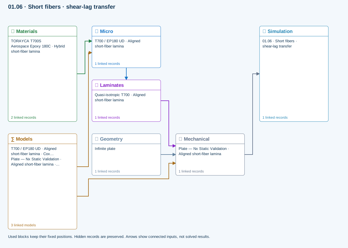
How information passes between models

Micro → Laminates: Predicted ply stiffness, strength, density and expansion properties.

Materials → Micro: Constituent stiffness, strength, density and thermal / moisture properties.

Mechanical → Simulation: SIMULATION selects this case and its analysis model; the case owns its applicable cycle and input references.

Laminates → Mechanical: Ply angles and thicknesses, stiffness, mass and ply properties.

Geometry → Mechanical: Part shape and dimensions, thickness or section definition, and model-specific geometric inputs. Each selected case consumes only the dimensions its model supports.

Models → Micro: Applied model assignment: Cox shear-lag elastic. Model parameters and formulation are used by Micro.

Models → Mechanical: Applied model assignment: CLT · Linear static with failure indices. Model parameters and formulation are used by Mechanical.; Maximum stress

Further reading and evidence

• Create and connect a lamina
• Edit material properties and units
• Run and review a model
• Review effective properties
• Connected inputs and result freshness
• Edit laminate materials, angles and thicknesses
• Related case study: NASA lamina analysis

Review the recorded validation scope. Retain the original inputs and solver notices with the results. Representative teaching data are not design allowables.