03.35 · Differential effective medium

An electromagnetic effective-medium calculation combines explicit electrical phase properties under a particular mixing idealization. This exercise examines what that idealization predicts and how its composition or architecture assumptions differ from simply assigning a mechanical composite record an electrical response.

Explicit dielectric teaching inputs. Mechanical laminate properties are not used in this separate RF study.

Open this exercise in Workbench

Prepare the baseline

Inspect the supplied phase permittivities, loss or conductivity inputs, frequency and fractions, together with any inclusion or interphase information required by the model. Establish the baseline before changing one supported parameter. Keep model-specific host, inclusion or symmetric-phase assumptions in your notes so that a comparison between formulations remains interpretable.

Worked procedure

1. Review the explicit electrical phase or layer properties and the frequency or excitation settings used by this EM study. Identify the conventions and assumptions stated for the selected formulation, including any geometry, fractions or layer thicknesses it requires. Do not substitute mechanical properties for missing electrical data; the model needs its own documented input basis.

2. Run the supplied study as a baseline and inspect the complete response curves, including their axes, units and parameter settings. Retain the numerical values or a clearly labelled capture before changing an input. Use the interpretation guidance below and the linked formulation to identify what each curve represents and which conclusions remain outside its scope.

3. Choose one editable parameter that belongs to this model and record its original and revised values. Keep the other inputs fixed, rerun the study, and compare the same output quantities over the same range. Explain the observed change using the linked formulation, including a discussion of whether the comparison stays within the model’s calibration and assumptions.

Review checkpoints

Do not interpret example calibration values as material allowables.

Record the assumptions and distinguish analytical verification from experimental validation.

Model limits

Incremental mixing with time-step refinement check. Positive-permittivity, passive, nonmagnetic RF screening only. This separate study uses explicit EM inputs, not mechanical or cure properties. Illustrative defaults are not measured T700 properties.

Interpret the comparison

Compare the relevant real and loss-related outputs using the displayed conventions and frequency. Explain the changed parameter’s role without assuming that all mixing laws describe the same physical architecture. Effective electrical properties require a deliberate handoff to a wave-propagation study; they are not inferred from elastic stiffness or automatically coupled to mechanical heating.

How information passes between models

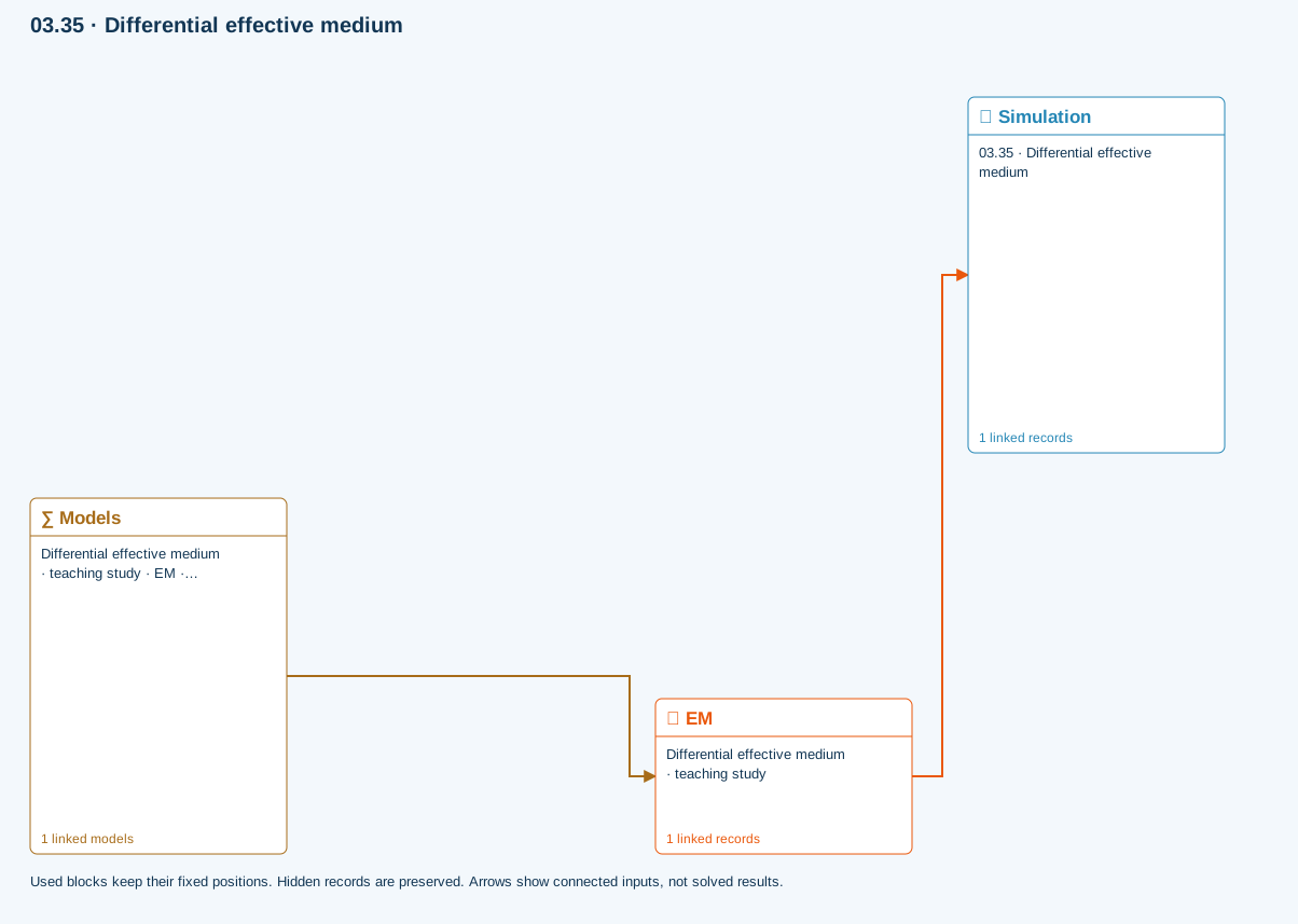
EM → Simulation: SIMULATION selects this case and its analysis model; the case owns its applicable cycle and input references.

Models → EM: Applied model assignment: EM · Differential effective medium. Model parameters and formulation are used by EM.

Further reading and evidence

• Advanced analytical models: equations, calibration and limits
• Edit laminate materials, angles and thicknesses
• Run and review a model
• Connected inputs and result freshness

Review the recorded validation scope. Retain the original inputs and solver notices with the results. Representative teaching data are not design allowables.