
The structural model turns laminate properties into a response for a particular geometry, load and support condition. Choose membrane, classical plate, shear-deformable plate, beam or cylinder equations according to the problem rather than treating their results as interchangeable.
Thin-plate theory neglects transverse shear deformation; first-order shear-deformation theory adds rotation and shear terms. A membrane cylinder and a layerwise thick-cylinder formulation represent different through-wall behavior. Apply the boundary conditions belonging to that model and distinguish distributed loads from force and moment resultants.
A stored process state can contribute to the structural response only through a supported coupling. State the reference temperature, reference moisture, stress-free condition and mechanical constraints. Tool-constrained stress, released residual stress and free curvature describe different states and should not be labeled as the same result.
Notch strength, viscoelasticity, bonded joints and shell stability add specialized assumptions and calibration data. A branch that uses the reference laminate stiffness does not automatically consume cure-dependent properties or progressive damage. Follow the linked technical formulation and the current implementation limits.
7.1 Plate, cylinder, and beam models
06.1 Manuals · read online, preview or download →
05.6.6 / Structural
Change the structural idealization without changing the shared material, micromechanics, laminate, process, or damage definition.
Set up lap shear, three-point bend, four-point bend and open-hole tension from Geometry →
Choose the structure
| Geometry ID | Idealization | Primary results |
|---|---|---|
| 1 | Rectangular laminate plate | Deflection, moments, buckling factor, natural frequency |
| 2 | Circular laminate cylinder | Radial/hoop/axial response using shell or Hyer formulation |
| 3 | Composite beam section | Centroid, I2/I3, EI, strain energy, deflection, buckling, frequency |
Plate boundaries
For the current Workbench plate module, choose Plate theory = CLT or FSDT in CASES. FSDT adds transverse shear and rotary inertia using shared laminate properties. Read the FSDT formulation, current scope and dedicated examples →
Geometry entries 8–11 assign the x0, x1, y0, and y1 edges independently: 1 simply supported, 2 fixed, or 3 free. Plate stiffness comes from the active laminate D matrix; mass and frequency use the calculated effective laminate density.
Cylinder formulations
Cylinder coordinates are axial x, hoop arc-length y, and radial z. Geometry entry 4 selects 1 for the engineering shell solution or 2 for the Hyer formulation. Pressure, axial force, and torque remain in the load-scaler group.
Beam sections
Geometry entry 12 selects rectangle, I section, circular tube, rectangular tube, or solid circle. The section dimensions occupy entries 14–21; end conditions occupy 22–23. The solver reports both geometric moments of inertia and laminate-effective EI.
Output interface
- The structural summary contains cylinder, plate, and beam section, response, energy, buckling, and frequency results.
- The cylinder load history contains pressure, force, torque, resultants, and radial traction.
- The cylinder stress-recovery table contains final radial coordinates and recovered stresses.
Engineering scope. These are reduced-order plate, cylinder, and beam calculations for sizing, comparison, and workflow integration. Validate boundary assumptions and model fidelity before certification or safety-critical use.
7.2 Shear-deformable laminated plates
06.1 Manuals · read online, preview or download →
Structural / FSDT
One laminate definition. Shared CLT stiffness. An integrated FSDT structural formulation.
Only blocks on the exercise path are shown. This changes the view only, not the exercise records.
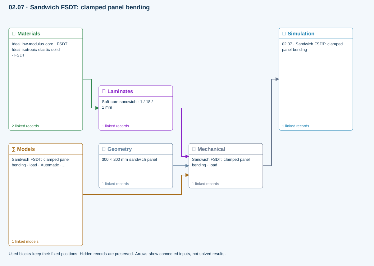
∑ Used models & submodels
Only models assigned to records used by this exercise are listed here. The full-layout option preserves the supplied starter records; no Workbench records are changed.
Automatic · Finite plate · Sandwich FSDT: clamped panel bending · load
Automatic selects FSDT for sandwich architecture and CLT otherwise. Static bending requires FSDT. Finite-plate studies do not consume process links or run progressive failure/fatigue.
Study · Static bending
Reference-elastic plate study; progressive failure and fatigue are not evaluated here.
Numerical settings
Ritz order: 6. Shear correction (FSDT only): Energy equivalent. Increase resolution to check convergence.
Data travelling between blocks
Materials → Laminates
Stored ply stiffness, strength, density and expansion properties.
Mechanical → Simulation
SIMULATION selects this case and its analysis model; the case owns its applicable cycle and input references.
Laminates → Mechanical
Ply angles and thicknesses, stiffness, mass and ply properties.
Geometry → Mechanical
Part shape and dimensions, thickness or section definition, and model-specific geometric inputs. Each selected case consumes only the dimensions its model supports.
Models → Mechanical
Applied model assignment: Automatic · Finite plate. Model parameters and formulation are used by Mechanical.
Where FSDT fits
Classical laminate theory supplies membrane, extension–bending and bending stiffness: A, B and D. First-order shear deformation theory (FSDT, or Reissner–Mindlin plate theory) retains those matrices and adds transverse shear flexibility. It does not generate a second set of constituent properties or replace the Micro model.
Sandwich plate default: new finite-plate analyses use Automatic theory. When the linked laminate Architecture is Sandwich Structures, Automatic resolves to FSDT; other architectures resolve to CLT. The choice is reevaluated when the linked laminate changes. Explicit CLT and FSDT selections are retained for comparisons. Use the default Energy equivalent shear correction for compatible sandwich plates. Missing shear properties or unsupported symmetry/geometry stop the run, rather than silently substituting CLT.
The three-point-bend sandwich beam example retains its separate shear-flexible beam and skin/core/bond screening model. Its concentrated load and failure checks are not replaced by the current uniform-pressure FSDT plate solver. FSDT completion does not establish a sandwich failure pass.
| Stage | Inputs and responsibility |
|---|---|
| Materials / Micro | Each ply supplies E1, E2, ν12, G12, G13, G23 and density. Stored materials and solved Micro plies can share the laminate. |
| Laminate | Angles and unequal ply thicknesses generate the common A/B/D matrices, transverse shear matrix As and thickness-integrated mass. |
| Geometry | Finite rectangular plate length and width. Thickness remains owned by the laminate. |
| CASES / SIMULATE | Select CLT or FSDT, study, edge restraints, pressure or reference membrane loads. One Run executes the chosen formulation. |
Kinematics and stiffness
u(x,y,z) = u0(x,y) + z θx(x,y)
v(x,y,z) = v0(x,y) + z θy(x,y)
w(x,y,z) = w0(x,y)
γxz = θx + ∂w/∂x     γyz = θy + ∂w/∂y
[N; M] = [A B; B D] [ε0; κ]
[Qx; Qy] = As [γxz; γyz]
Rotations are independent of the displacement slope. The thin-plate limit drives transverse shear strain toward zero. The current CDS plate release solves w, θx and θy for symmetric reference-elastic laminates; it rejects non-negligible B coupling rather than discard in-plane/bending coupling. A/B/D are calculated by the same laminate implementation used by CLT.
Transverse shear properties
FSDT requires positive G13 and G23 for every ply. An isotropic stored material may derive them from its isotropic shear modulus; orthotropic records need directional data. Missing values cannot be replaced silently by G12.
- Energy equivalent: the default directional pure-bending approximation integrates equilibrium shear profiles through all plies, matches their shear strain energy and inverts the resulting 2×2 flexibility. It requires symmetric, specially orthotropic bending stiffness (D16 and D26 negligible). It recovers 5/6 Gh for a homogeneous section while accounting for a soft core.
- Uniform 5/6: explicitly applies 5/6 to the integrated rotated shear stiffness. This is a homogeneous-reference approximation, not a universal correction for sandwich or strongly heterogeneous laminates.
Directional energy approximation:
qi(z) = −∫(bottom→z) Q̄ii(s) s ds / Dii
Cs,ij = Σlayers ∫ qi(z) [Ḡs(z)⁻¹]ij qj(z) dz
As = Cs⁻¹

Uniform approximation:
As = (5/6) Σlayers Ḡs,k tk
The directional approximation is not a complete 3D stress recovery or a universal anisotropic warping solution. Its limits remain visible in results. As is reported in N/mm; Qx and Qy are integrated shear force per unit width, not interface stress.
Studies and boundary conditions
- Static bending: FSDT with uniform Plate pressure in MPa (= N/mm²). Clear Nx, Ny and Nxy. Outputs include physical w in mm, rotations in radians, Qx/Qy in N/mm, cursor sections, sampled peak |w| and the shear share of elastic energy.
- Modal: unprestressed, undamped frequencies. Through-thickness density integration includes rotary inertia I2 = ∫ρz² dz. Explicit positive density and symmetric mass distribution are required.
- Buckling: elastic bifurcation under uniform proportional Nx, Ny and Nxy. Negative normal resultants mean compression. The multiplier scales that load vector; it is not a strength or postbuckling limit.
| Edge | FSDT restraint |
|---|---|
| Simply supported | w = 0 and tangential rotation = 0; normal bending moment is natural. This is the hard simply supported convention. |
| Clamped | w = θx = θy = 0. |
| Free | Natural moment and transverse shear conditions; no essential displacement restraint. |
Numerical method and applicability
CDS uses a polynomial Rayleigh–Ritz formulation with independent displacement/rotation fields, enriched rotation spaces and exact-enough Gaussian integration for the polynomial products. Ritz order 4–8 controls spatial approximation. Refinement is essential, particularly for clamped edges, thin plates, soft cores and higher modes. A small algebraic residual does not establish spatial convergence.
The FSDT release accepts thickness / shorter side up to 0.2 as an implementation guard, not a universal accuracy guarantee. It excludes holes, thickness stretch, geometric nonlinearity, process residual preload, damping, contact, unsymmetric extension–bending coupling and mass coupling. Buckling and modal runs do not consume transverse-pressure preload. Extremely thin plates may be better conditioned with CLT.
No false failure pass. FSDT improves global response but does not establish interface peel stress, bond strength, delamination growth, core crushing or ply failure. Those require separately supported constitutive and interface models. The current FSDT release cannot be combined silently with the layerwise progressive-damage or delamination solver.
Try the dedicated exercises
These six examples are part of the shared default database and the searchable curriculum. They use idealized teaching properties, not qualified material allowables.
- Thick isotropic plate — static bending and thickness sensitivity ↗
- Cross-ply plate — CLT/FSDT buckling and frequency comparison ↗
- Soft-core plate — transverse shear and correction sensitivity ↗
- Sandwich panel — clamped uniform-pressure bending ↗
- Sandwich panel — biaxial compression buckling ↗
- Sandwich panel — directional-core natural frequencies ↗
Find these examples by searching FSDT or selecting the FSDT model →
Sandwich exercise sequence
Find these four studies under 07 · Sandwich FSDT in the default database simulation tree, or filter the exercise manual by FSDT and sandwich application. All use symmetric 1 / 18 / 1 mm skin–core–skin stacks, explicit shear properties and Automatic → FSDT. The unchanged teaching materials are shared; duplicate a record before making an independent variant.
| Exercise | Baseline setup | What to inspect |
|---|---|---|
| fsdt-03 · Shear-dominated bending | 200 × 200 mm; simply supported; 0.001 MPa uniform pressure | Physical deflection and shear-energy fraction; compare shear corrections. |
| fsdt-04 · Clamped panel bending | 300 × 200 mm; all edges clamped; 0.001 MPa uniform pressure | w, rotations and Qx/Qy cursor sections; compare simply supported edges and pressure scaling. |
| fsdt-05 · Biaxial buckling | 300 × 200 mm; simply supported; Nx = −1000 N/m, Ny = −500 N/m; pressure zero | First positive multiplier and proportional critical load pair; compare uniaxial compression and CLT. |
| fsdt-06 · Directional-core modes | 300 × 200 mm; simply supported; all applied loads zero; core G13 = 0.025 GPa, G23 = 0.0125 GPa | First three frequencies and normalized mode shapes, including rotary inertia; exchange core shear directions. |
For every study, refine Ritz order from 6 to 8 and record convergence before interpreting trends. These are idealized elastic teaching problems, not strength allowables or experimentally validated sandwich designs. Biaxial buckling is not a wrinkling, bond or core failure criterion; natural-frequency mode amplitudes are not physical vibration displacements.
Verification and validation
Automated module checks compare homogeneous shear stiffness with 5/6 Gh, simply supported static displacement with an independent double Fourier series, buckling with the shear-flexible Navier solution, and frequency with a rotary-inertia eigenvalue reference. Tests also check convergence toward CLT, clamped-edge refinement, required-property errors and the production data definition. These are analytical software verification, not experimental validation or validation of every exercise variation. Dedicated example results are not automatically given a full-model benchmark badge.
Primary references
- FEniCS-Shells: laminate ABD and Reissner–Mindlin shear stiffness — the separation between common laminate stiffness and transverse shear stiffness.
- FEniCS-Shells: clamped Reissner–Mindlin plate — independent rotations, shear energy and the need to control shear locking. CDS uses Ritz approximation, not this finite-element implementation.
- Abaqus theory: transverse shear stiffness in composite shells — energy-equivalent shear concepts and layered-section limitations. CDS's directional approximation is not identical to Abaqus's formulation.
7.3 Constant-section shell cylinder
06.1 Manuals · read online, preview or download →
05.6.02 / Structural / Cylinder model 1
Resolve pressure, axial force, and torque through a laminate membrane-shell idealization with a constant circular section and the shared CDS laminate property definition.
Scope and coordinates
Current Workbench pressure summary. The thin-wall pressure strain summary uses the complete inverse laminate extensional stiffness, including Poisson and extension–shear coupling: ε⁰ = A⁻¹N with curvature constrained to zero. Its x direction is axial and y is hoop. Open ends omit the pressure end-cap force, but axial Poisson contraction remains. This summary is not the general free-curvature ABD shell solution shown below, and it does not resolve radial stress or local end effects. Keep the separate layerwise thick-wall profile and supported ply-failure calculations distinct.
The shell route uses axial x, circumferential arc-length y = rmθ, and outward radial z coordinates. It is intended for thin-to-moderately-thick cylinders where a membrane-dominant sizing solution is appropriate. The laminate ABD matrix, environmental resultants, damage state, and density come from the same upstream solver used by the plate and beam branches.
Equation detailsExplanation · variables · model connection · reference+
Converts the pressure difference across a closed-end cylinder into hoop and axial membrane force per unit length.
Model connectionThese pressure terms enter the common laminate resultant vector before constitutive recovery.
Theory basisCDS online structural theory, structural geometry module
Equation detailsExplanation · variables · model connection · reference+
Superimposes user-applied axial force and torque on the pressure-generated membrane actions.
Model connectionThe load-scaler inputs remain independent of geometry and are transformed into the shell resultant basis here.
Theory basisCDS online structural theory, cylinder loading
Equation detailsExplanation · variables · model connection · reference+
Uses the active laminate ABD matrix to recover mid-surface strain and curvature after mechanical and environmental resultants are combined.
Model connectionRecovered ply strains and stresses feed the selected failure and progressive-damage models.
Theory basisCDS hygrothermal CLT and ABD theory
Radial response and outputs
For the membrane shell path, the mean radial displacement is recovered from the hoop strain as w ≈ rmεy. Named results provide the cylinder summary, pressure, force, torque and resultant histories, plus the final radial-coordinate and recovered-stress table.
Assumptions and limits
- Axisymmetric constant circular section with small strains and small displacement.
- Membrane-dominant response; local end effects, ovalization, openings, and geometric imperfections require higher-fidelity analysis.
- Closed-end axial pressure force is included only when the selected end condition requires it.
- Use the Hyer route when through-wall radial stress and layer-interface traction continuity are important.
7.4 Hyer thick laminated cylinder
06.1 Manuals · read online, preview or download →
05.6.03 / Structural / Cylinder model 2
Resolve the radial coordinate explicitly through every ply so pressure tractions, interlaminar stress, and displacement continuity are retained across a thick laminated wall.
Methodology
The Hyer route follows the generalized-plane-deformation treatment for long laminated cylinders. Each concentric orthotropic ply is transformed into the axial–hoop–radial coordinate system. The solver constructs a layer solution, enforces radial equilibrium inside each ply, applies displacement and traction continuity at every interface, and closes the system with inner and outer pressure boundary conditions.
Equation detailsExplanation · variables · model connection · reference+
Defines the axial, hoop, and radial strains for an axisymmetric cylinder with generalized uniform axial extension and layerwise radial displacement.
Model connectionThese kinematic fields are evaluated separately in each ply while sharing interface displacement constraints.
Theory basisHyer (1988), stress analysis of thick laminated cylinders
Equation detailsExplanation · variables · model connection · reference+
Relates the three-dimensional stress state in each transformed orthotropic ply to mechanical strain after thermal and moisture free strains are removed.
Model connectionThe pristine or damaged per-ply property source is resolved upstream and passed unchanged into this layerwise cylinder branch.
Theory basisCDS independent per-ply material routing
Equation detailsExplanation · variables · model connection · reference+
Enforces axisymmetric equilibrium through the wall so radial and hoop stress are mechanically compatible in every ply.
Model connectionThe resulting ordinary differential system determines each layer's radial solution coefficients.
Theory basisHyer (1988), radial equilibrium formulation
Equation detailsExplanation · variables · model connection · reference+
Closes the multilayer system by preserving radial displacement and traction at ply interfaces and applying pressure tractions at the inner and outer radii.
Model connectionCDS assembles these equations and conditions into one linear coefficient system for the active laminate wall.
Theory basisHyer (1988), layer and surface conditions
Recovered results
The model recovers radial displacement and the axial, hoop, radial, and interlaminar shear stresses at requested through-wall positions. Named results provide the load and resultant histories plus the final radial-coordinate and stress-recovery table.
Selection guidance
| Use shell cylinder when | Use Hyer cylinder when |
|---|---|
| Rapid sizing, membrane dominance, and large radius-to-thickness ratio | Thick walls, strong radial gradients, or interface tractions matter |
| Hoop/axial resultants are the primary design quantities | Layerwise radial displacement and interlaminar stress are required |
Verification basis. Check single-layer isotropic limits, traction continuity, pressure boundary recovery, equilibrium, and convergence of through-wall sampling before using the layerwise solution in design decisions.
7.5 Process fields in progressive laminate failure
06.1 Manuals · read online, preview or download →
05.6.4 / Structural
Map temperature, moisture, cure shrinkage, and crystallization shrinkage into each ply, form their laminate resultants, and superimpose them with static or progressive mechanical loading. Expand any equation for its physical meaning, variables, units, model connection, and theory source.
Enabled local free strains
Equation detailsExplanation · variables · model connection · reference+
Adds the unconstrained strain caused by temperature change, moisture change, thermoset chemical shrinkage, and thermoplastic crystallization shrinkage. Independent binary switches let each contribution enter or leave the structural solve without changing the process solution.
Model connectionEvaluated at mapped bottom, middle, and top structural recovery points for every ply. These are the same free strains subtracted during stress recovery and failure evaluation.
Theory basisNASA hygrothermal laminate mechanics
Equation detailsExplanation · variables · model connection · reference+
Rotates each local engineering free-strain vector from material axes 1–2 into laminate axes x–y using the ply orientation.
Model connectionThe transformed field is multiplied by the ply’s damaged transformed stiffness Q̄d when process force and moment resultants are integrated.
Theory basisClassical lamina transformation relations
Mapping the process mesh to three structural nodes per ply
The transport mesh may contain any user-selected number of cells per ply, whereas structural visualization and field output retain exactly three recovery nodes per ply. R15 least-squares fits each process field to a linear function within its owning physical ply, then evaluates that fit at the bottom, middle, and top coordinates.
Equation detailsExplanation · variables · model connection · reference+
Finds the best constant and gradient for temperature, moisture, cure shrinkage, and crystallization shrinkage within one ply from all transport cells belonging to that ply.
Model connectionPreserves both the ply-average process state and its first through-thickness gradient while keeping the stress/strain field histories and animation mesh fixed at three structural nodes per ply.
Theory basisReduced-order process-to-structure mapping
Damaged laminate stiffness and process resultants
Equation detailsExplanation · variables · model connection · reference+
Integrates the current transformed stiffness of every ply through the laminate thickness. Progressive failure changes Q̄d and therefore rebuilds A, B, and D.
Model connectionThe same damaged stiffness used for mechanical equilibrium also weights the process resultants, so a new ply failure changes load redistribution and residual-stress restraint at the same accepted load.
Theory basisNASA classical laminate ABD formulation
Equation detailsExplanation · variables · model connection · reference+
Converts an otherwise free process strain into equivalent in-plane forces and moments representing the restraint imposed by the bonded laminate. A gradient contributes directly to process bending moment.
Model connectionRecomputed after any new damage state before same-load re-equilibration. The process-resultant history reports each component over the structural increments.
Theory basisHygrothermal force and moment resultants
Combined generalized equilibrium
Equation detailsExplanation · variables · model connection · reference+
Solves simultaneously for mid-plane strains and curvatures under the sum of enabled mechanical and process-equivalent resultants. This is the governing superposition step, not a postprocessed stress offset.
Model connectionUsed for a static mechanical state or at every progressive load increment. The mechanical-load flag may remove Nmech and Mmech while retaining process-only residual response.
Theory basisNASA generalized laminate equilibrium
Equation detailsExplanation · variables · model connection · reference+
Recovers the compatible global strain at any z and subtracts the enabled free strain before applying the current damaged stiffness. The result is the actual constrained ply stress used by failure criteria.
Model connectionEvaluated at the bottom, middle, and top of every ply and then transformed to local 1–2 axes. Top and bottom surface states govern the progressive failure check.
Theory basisClassical laminate stress recovery with hygrothermal strain
Equation detailsExplanation · variables · model connection · reference+
Reports total fields together with separately evaluated mechanical, thermal, moisture, cure-shrinkage, and crystallization-shrinkage contributions at the same increment and damaged material state.
Model connectionSupports the global, local, principal, and process-only field histories so CDS can display each contribution without reconstructing it outside the solver.
Theory basisProcess-induced residual-response decomposition
Progressive same-load update
At each accepted increment the solver recovers all three structural nodes per ply; checks both surfaces; evaluates the independent criterion assigned to that ply; degrades only newly activated stiffness families; rebuilds damaged ABD and process resultants; and re-equilibrates at the same combined mechanical–process load until no new event occurs.
Coupling boundary. The process solver is one-way with respect to structural damage in r15: process fields create structural strains and stresses, while ply damage changes the stiffness that restrains those fields. Damage does not yet change k3, cp, diffusivity, cure kinetics, or crystallization kinetics.
Auditable outputs
- Stress and strain histories: total, mechanical, thermal, and moisture contributions.
- Transport histories: mesh, fields, state, rates, heat, shrinkage, and surface interpolation.
- Structural process mapping: mapped states and active physical components.
- Process-only fields: global and local stress and strain.
- Process resultants: force and moment components at every structural increment.
Theory references
7.6 Move from laminate mechanics to structural decisions.
06.1 Manuals · read online, preview or download →
Theories / Structural
Connect idealization, mechanical and process loading, residual stress, recovered fields, independent ply failure, damage progression, structural outputs, and verification.
Theory map
Models, equations, figures, and cross-referencesLaminate to structure
Carry the ABD property definition and recovered ply response into plates, cylinders, and beam sections.
Open structural framework →Constant-section shell cylinder
Resolve pressure, axial force, and torque as membrane resultants using a laminate shell idealization.
Open shell-cylinder theory →Hyer thick laminated cylinder
Resolve layerwise radial displacement, through-wall stress, traction continuity, and generalized plane deformation.
Open Hyer-cylinder theory →Response, failure, and verification
Combine structural fields with process residuals, failure measures, output interfaces, and verification checks.
Open geometry models →Complete reference
One continuous sequenceStructural framework
→02Constant-section shell cylinder
→03Hyer thick laminated cylinder
→04Process-to-structural coupling
→05Plate, cylinder, and beam models
→06FSDT shear-deformable plates
→07Fatigue S–N models
→08Advanced analytical studies
→09ASTM Virtual Test Lab
→10Failure assessment
→11Verification and validation
→7.7 Bonded roller contact · width variants
In Geometry, choose Roller, select the core metal and coating elastomer, and enter outer radius and coating thickness. Set Width condition and Roller width there. A roller is an auxiliary geometry element: adding, selecting or editing an unconnected roller does not create a load case, replace the specimen geometry, or change the active simulation. The usual geometry-driven case selection applies to specimens, not rollers. For an optional roller assessment, explicitly create a Rubber-covered roller contact case in Cases, select the roller in its Geometry input, and connect that case to a separate Simulation. Set force and contact condition there. An explicitly linked contact case or thermal-process roller station uses the roller width condition to choose its solver variant.
| Geometry choice | Calculation | Meaning of Roller width |
|---|---|---|
| Infinite width | Fast analytical elastic-layer fields with a numerical 2D contact solve. Plane strain: axial displacement and strain are zero. No free-end spreading. | Reference loaded span used to convert total force into line load F/width. It does not introduce physical ends into the calculation. |
| Finite width | 3D small-strain elastic contact. The two free rubber ends can bulge and spread axially; pressure varies across the width. This takes longer. | Full physical axial width of both rubber and core, uniformly pressed against the rigid flat. |
The rubber is perfectly bonded to the rigid metal core: no slip or separation at that interface. Changing width mode retains material choices, radius, thickness, width and load. Old records with only a case-level Roller face length retain that reference span in Infinite width until a width is entered in Geometry. Finite width always requires its dimension in Geometry.
Coating color, hollow cores and shafts
In Materials & coating, use the silicone color swatches or Custom color picker. Color is saved with the geometry and shown on the 3D surface, radial section and material legend. It changes appearance only, not material properties or contact results.
The geometry editor keeps relevant fields in one compact table. Use the information icon beside a field for its explanation. Calculated dimensions and More details expand below the inputs. Inactive bore, shaft and wall controls stay hidden while their saved values are preserved.
Core construction offers Solid core, Hollow core or Core with shaft. Hollow core adds Core bore diameter: a through hole smaller than the core outer diameter. The preview shows the opening and metal wall thickness. Core with shaft adds Shaft diameter and Shaft overall length. The shaft uses the selected core metal and is centred in the roller.
Shaft overall length is the full end-to-end dimension, including the coated Roller width. Each exposed end is (Shaft overall length − Roller width) / 2. For example, a 100 mm roller with a 150 mm overall shaft has 25 mm exposed at each end. Shaft diameter cannot exceed the core outside diameter. Roller width defines the loaded width for standalone contact and finite-width process rollers. In a thermal process, Infinite width uses the plate width as its loaded span. Shaft length never replaces the contact span.
Only dimensions for the chosen construction appear. Switching construction preserves the hidden values for reuse, and switching away from Roller and back preserves the whole configuration. The contact solver still assumes a perfectly rigid core: hollow-wall flexibility, shaft bending and bearing support are not predicted. Infinite width still means plane-strain coating response even when the preview includes a shaft.
Results and controls
Both variants give contact pressure, nip width, indentation, coating stress, strain and displacement. The finite variant adds the contact footprint across the width, axial displacement v, axial strain εy and end bulging. In the axial panel, choose Across width at the nip centre or Free end along the nip. Field selectors change the contour quantity. Mesh magnification changes display only. Field CSV exports the centre section; Axial fields CSV exports the half-width axial section and free end in mm, MPa and dimensionless strains.
Friction
Friction applies only between outer rubber and the rigid flat. Frictionless means no tangential traction; Sliding +x or −x prescribes traction on rubber q = ±μp. A friction coefficient alone cannot determine partial slip or free rolling. No adhesion, rolling resistance, heating or time-dependent rubber response is inferred.
Equations, convergence and limits
x follows the nip, y is the roller axis and z points into the coating. Both variants approximate the curved coating locally as a flat bonded layer, with initial contact gap x²/(2R). The long-roller solver uses Fourier/Airy elastic modes and force-balanced nonnegative contact pressures.
The finite solver uses 3D eight-node B-bar bricks: full integration of deviatoric elasticity and mean volumetric strain to reduce near-incompressible locking. The core boundary has u = v = w = 0. Symmetry at y = 0 fixes only v; the outer end is traction free. Distant x boundaries are fixed, six coating thicknesses or more from the nip centre. Contact is solved with a finite penalty, active contact set and total-force balance. A second mesh must change indentation and maximum outward end displacement by less than 5%. This check does not establish convergence of sharp-edge peak pressure or stress. Stress/strain contours recover volume-weighted element-centre fields.
The coating must be thin relative to the radius (h/R ≤ 0.2), contact extent small (a/R ≤ 0.15), and strains and indentation/thickness within 15%. The core modulus must be at least 100 times the coating modulus. These are screening limits, not accuracy guarantees. Finite width requires measured Poisson ratio below 0.5; exactly incompressible rubber needs a mixed-pressure model. Large deformation, hyperelasticity, core bending, end caps, crown, tilt and imperfect bonding are excluded.
Numerical checks cover constant-strain elasticity, rigid motion, contact force equilibrium, bonded displacement, free-end spreading symmetry, friction reversal, mesh/domain/penalty sensitivity, and the wide-roller approach to the plane-strain result. These are numerical checks, not experimental validation for a specific rubber compound.
Wide roller · film traction and buckling
In the contact case, set Film assessment to On. These controls appear only with Infinite width geometry. Film assessment is Off by default. Switching to Finite width retains the entries but excludes film traction and buckling screening from the run; switching back restores them.
Film thickness, modulus and Poisson ratio describe an isotropic elastic film passing through the nip. Film width is the film span across the roller axis, no larger than the geometry reference width. Entry tension is total force across that film width. Roller speed and web speed are signed in the +x direction; Slip speed smooths the transition around zero relative velocity. Equal velocities produce zero traction in this regularized sliding model, not a static-friction solution.
The film friction law is μ(p) = min(μcap, max(0, μ0 + gain ln(1 + p/pref))). Set pressure gain to zero for constant friction. Traction on the film is τ = μ(p)p tanh((vroller − vfilm)/vslip). The membrane force balance is d(σx h)/dx = −τ. Entry tension is specified; exit tension is predicted. The earlier linear exit-stress adjustment is deliberately omitted because it changes stress without adjusting traction. These film tractions are a one-way assessment using the pressure; they do not recalculate rubber displacement or its separate outer-surface friction loading.
Positive stress is tensile; negative stress is compressive. Film strain is σx/E before buckling. Film rigidity D = Eh³/[12(1−ν²)]; critical compressive stress σcr = kπ²D/(b²h). Film buckling coefficient k describes assumed support conditions. Film effective span b accepts a positive physical unsupported span, or zero for the source-inspired nip estimate: the extent above 2% peak pressure, bounded to 0.5–25 mm. The estimate uses panel edges; the earlier estimate used sample centres.
Buckling index is max(0,−σx)/σcr. One means the screening threshold is reached. The factor is σcr divided by maximum compressive stress; with no compression it is reported as No compression. Contact fraction above threshold measures length within contact above 1% peak pressure; it is also the area fraction under the uniform-width assumption. The graph selector offers stress, strain, film traction and buckling index. Film CSV exports all four, pressure, friction, critical stress and effective span.
This unsupported-plate estimate is not a validated supported-nip instability calculation. No wrinkle wavelength/amplitude, nonlinear film state, postbuckling, rubber buckling, or feedback of film deformation into contact is predicted. Negative exit force means the imposed speed/tension combination demands compression and needs a postbuckling/contact model to determine its realized state.
Adapted elements: pressure-dependent friction, regularized slip, film membrane equilibrium and plate-buckling screening from the supplied silicone_roller_contact_MASTER_V4_FILM_TRACTION_BUCKLING.m. The supplied Silicone Roller Pressure Model_v2.pdf describes local hyperelastic foundations and explicitly excludes exact bonded lateral constraint; those foundation laws have not replaced the bonded elastic-layer solver.
Moving thermal process · roller boundaries
Open the thermal case, set Process mode to Moving Process, then open Upper or Lower. Select a Plate or Rectangular section workpiece. Choose a roller ID directly in a row’s Boundary condition dropdown. Create your rollers in Geometry first; adding a geometry alone never changes the process. Add a row at each desired contact centre. Up to 12 roller assignments are supported; the same geometry can be reused at several locations with independent force and temperature. The separate Rollers tab is no longer needed.
| Control | Function |
|---|---|
| Boundary condition / roller ID | Selects core, elastomer, radius, coating thickness and width variant. Its material links travel with the simulation. |
| Upper / Lower tab | Chooses the surface. Opposed rollers may share a centre. |
| Position / centre (m) | The row location is the nip centre, measured from the inlet. Its edges are predicted from roller geometry, material and force, independently of spacing between rows. At the inlet/outlet only contact within the scheduled travel is applied. |
| Coordinate | Length enters centres in metres. Time enters arrival times in minutes, with x = velocity × time. Switching coordinates preserves physical centres. Changing velocity in Length mode changes dwell time; in Time mode it changes centre locations. |
| Contact settings button | Opens temperature, conductance, pressure dependence and outside-contact settings beside the chosen roller. Force is entered directly in the table. |
| Applied load | Roller rows show Force (N): the total normal force on that roller. Contact pressure and nip width are calculated from this force, roller geometry and the active contact material properties. Ordinary rows show Pressure (MPa). Values are stored separately; changing boundary type never converts pressure into force. |
| Roller (°C) | Prescribed surface temperature, or initial roller temperature when Rotating thermal model is selected. |
| h (W/m²·K) | Thermal contact conductance at the reference pressure. The initial 1000 is an editable example, not a calibrated prediction. |
| Pressure exponent / reference pressure | Optional contact law h = h_ref (p/p_ref)^n. Default n = 0 gives constant conductance; p_ref is in MPa. Use measured or justified values. |
| Outside contact | By default, Follow profile interpolates the background from neighboring ordinary rows; the roller centre is not a background knot. Select Custom to use its saved boundary type, environment temperature and shared background pressure as an explicit point. Background pressure remains additive and can be edited here. The main temperature cell becomes roller temperature; it is not interpolated into surrounding environmental temperatures. |
| Remove roller / row | Choose an ordinary boundary condition to remove just that face’s roller. Deleting a row removes its upper and lower roller assignments. Roller geometry is retained; normal undo and record save apply. |
| Fill boundary down / Copy to opposite surface | Copies the selected boundary and roller settings to subsequent rows or the opposing face at the same centre. Added rows do not automatically inherit a roller. Overlapping same-face nips are rejected when solving. |
Older saved station positions are shown as boundary rows without changing the background temperature or pressure profile; edits save their row bindings. Normal record copying and snapshots retain roller geometry references and boundary settings.
Pulling velocity maps position to time: x = vt. Each roller uses its selected coated or metal contact model to predict its nip pressure. Upper and lower roller pressure are independently added to the existing cycle pressure. The contact heat flux is h times the difference between roller and surface temperatures. It replaces the ordinary thermal boundary over the covered area while that part of the workpiece passes through the nip; the uncovered area retains the existing boundary.
The Upper/Lower editor uses compact Workbench rows, with the Pressure & temperature plot to the right. Drag the divider to resize the table and plot. The plot remains available before a roller is assigned, showing the background schedule. Boundary settings holds the face’s film coefficient and its existing lock control; it applies to background convection/tool contact, while roller contact uses its own conductance. Process settings holds die length and the inlet/outlet assumptions; mode and speed remain in the toolbar. LiveLoad also shows the combined plot. Contact pressure is recalculated in the background from the current force, geometry and material properties. The plot uses °C on the left and MPa on the right, with one shared pressure curve and a dashed global-pressure line. Both tables and the material models use this same through-thickness pressure. It is the global profile plus the largest active roller contribution at each position; opposing pressures are not added. This is a 1D pressure-envelope approximation, not a coupled roller equilibrium solution. Outside a roller’s predicted nip its contribution is zero. The pointer readout shows global + roller = total, and selecting a roller in the zoom list shows this breakdown at its centre. Shaded bands mark predicted nip widths. Choose a roller in the zoom list to inspect its narrow pressure profile. Moving the pointer shows sampled values; Plot CSV exports the full process. When inputs change, the previous prediction is hidden while recalculating.
Thermal results include the same combined plot for the saved run, plus Roller boundary history. Choose pressure, conductance or boundary temperature; zoom to a station and export Boundary CSV. The station table reports nip width, local peak pressure, entry/exit time and force-balance error. Pressure curves are averaged across workpiece width, so local finite-roller peak pressure differs from the plotted average. The time solver resolves individual nip panels even when the normal output interval skips the contact; additional snapshots are saved across each nip.
Supported scope and assumptions
Infinite-width process rollers span the full workpiece width with uniform coverage across it. Their line load is total applied force divided by workpiece width; the saved geometry width remains available for standalone contact. Coverage along travel is still limited to the predicted nip. Finite-width rollers use their actual width, are centred across the plate, and may not exceed the workpiece width. Same-side nips may not overlap. Roller forces and thermal conditions remain independently prescribed. The shared pressure envelope is not an equilibrium solution for a freely bending web. The workpiece is locally a rigid flat for contact and a through-thickness thermal section for heating. A partial-width contact is averaged across the workpiece; lateral and axial temperature gradients are not resolved. A full-width infinite roller can replace a prescribed-temperature background during nip contact and restore it outside the nip. Partial-width finite rollers require convection, tool contact or insulation on that face; a prescribed-temperature background cannot represent that mixed condition. A width-mismatch message reports plate width and actual roller coverage.
Pressure supplies a boundary history and the optional contact-conductance law. It does not automatically solve compaction, resin flow, thickness change or plate deformation. Prescribed-temperature mode does not include roller heat capacity. Rotating thermal mode adds roller heat storage and conduction. Frictional heat, rate-dependent rubber behavior, temperature-dependent contact stiffness and film buckling remain excluded. The separate wide-roller film assessment remains available in its standalone case. Contact conductance needs its own calibration; rubber pressure alone cannot determine it.
Thermal contact conductance and interface heat transfer background
Rotating roller heat transfer
In a roller row, open Contact settings and choose Rotating thermal model. The row temperature becomes its initial temperature. By default RPM = web speed / circumference, with consistent metre/minute units and no slip. Machine age at web entry controls how long the roller has already operated when the analyzed strip enters. It is separate from that strip’s travel time. Set the surrounding air temperature and film coefficient, plus optional absorbed irradiation outside the nip.
The solver tracks temperature around the circumference and through radial metal/coating layers. Rotation transports the stored heat; conductivity redistributes it, and density × specific heat determines storage. The predicted nip and conductance supply the contact arc. Constant thermal properties come from the selected core and elastomer materials. No heat is generated merely by rotation.
During contact the boundary is h(Tweb − Troller). Outside contact it is hair(Tair − Troller) plus absorbed flux. The hollow bore is insulated and removes the corresponding thermal mass; shaft extensions and axial/end heat losses are excluded. Both coated and all-metal rollers are supported. Infinite-width geometry uses the workpiece span; finite rollers use a width-averaged thermal cross-section, not a 3D end-temperature solution.
The plate and roller temperatures are iterated to a 0.1°C contact-temperature tolerance. Warm-up uses one fixed contact-web temperature from the selected moving-web solution, representing continuous feed at approximately stationary process conditions. This is not a simultaneous startup simulation of every strip in the line. The existing pressure model does not change with roller temperature. Friction and rubber hysteresis heating are not included.
Thermal results show contact, mean-surface and core temperatures against machine running time, plus RPM, surface range, energy residual and Thermal CSV. The input preview continues to show initial temperatures until Run. The 72 angular × 16 radial cell model conserves energy but averages very narrow nips; local flash-temperature predictions require a finer dedicated contact model.
Live Process · 3D boundary view
For a moving thermal process, open Upper or Lower and choose Live Process beside Pressure & temperature. Both surfaces, zones and rollers appear together and update when the boundary rows, forces or geometry definitions change. Roller centres follow their row positions. The continuous workpiece spans the scheduled travel distance; it is not an animation of a finite coupon.
Solid plate shows the workpiece as one body. Layered laminate uses its assigned laminate, actual ply thicknesses and material finishes. Link a laminate to the thermal case or workpiece to enable this option. All dimensions use a common scale. Finite rollers retain their coating color, face width, core and shaft dimensions. Infinite rollers are drawn across the plate width.
Drag to rotate, Shift-drag to pan, and scroll to zoom toward the pointer. Double-click a zone or roller to fit it, or empty space to magnify it. The + / − controls and percentage selector also change zoom. Side and Top provide fixed starting views. Expand opens a larger window; Fit selected frames the selected zone or roller; Fit whole process resets the view. Keyboard arrows rotate and Home resets. Select an object or use the inspection dropdown to read its details. Callouts adds labels on the scene; All zones & rollers expands the full list. SVG saves the current view.
Zones show the upper and lower boundary conditions, programmed temperature ranges and global pressure. Rollers show applied force, prescribed surface temperature, contact conductance, dimensions and predicted nip / peak pressure. Red arrows indicate force direction and red strips indicate predicted contact footprints. These are boundary inputs and contact predictions, not solved interior temperatures or a deformed plate. Incomplete contact inputs produce a pressure-preview message while retaining the geometry view.
Live Process boundary symbols
Symbols shows each zone’s upper and lower boundary types and roller contact locations. Curled air lines indicate convection; opposed red/blue arrows indicate contact heating or cooling; a thermometer indicates prescribed temperature; a hatched surface indicates insulation. Symbols are schematic and do not specify airflow, equipment size or solved heat-flow direction.
Open Boundary symbol key & annotations and select a zone. Its Upper and Lower selectors default to Auto, following the actual boundary inputs. You can choose a symbol-only annotation for convection, contact, radiation or the planned laser-heating model. Radiation uses wavy rays; laser uses a beam and spot. Annotations are shared with the expanded view during this view session and do not change saved boundary conditions. Radiation is not separately solved by the current film law, and selecting a laser symbol does not activate a laser solver.
All-metal rollers
In Geometry → Roller materials, set Roller surface to All metal. Select steel (or another metal) in Core metal. Roller outer radius now describes the metal surface; the derived outer diameter is twice this radius. Coating material, thickness and color are hidden and retained if you switch back.
Metal contact model offers Elastic metal fields and Hertz pressure only. Both predict the same elastic Hertz pressure against a rigid flat from force, radius, loaded width and the selected metal’s modulus and Poisson ratio. Elastic metal fields also shows local stress, strain and displacement; its sliding traction is a one-way calculation that does not alter the normal pressure. Hertz pressure only is the faster frictionless option.
Model limits and deformation reference
These are local line-contact models, including for finite-width metal geometry. They do not predict axial end spreading, shaft bending, hollow-shell ovalization, plasticity or bearing compliance. The half nip must be at most 5% of radius, loaded width at least ten nip widths, and metal depth at least eight half nips. The displayed field extends eight half nips into the metal; this is not a fixed core boundary. Displacements use a datum at the bottom centre of that local field. Geometric nip flattening is a²/(2R), not the total approach of the roller shaft. Verify the elastic assumption against the selected material’s yield limits.
Select the roller ID in a moving thermal boundary row as usual. Enter force in N. Its calculated pressure is added to the global pressure over the predicted nip; temperature and contact conductance remain the boundary-row settings. Finite-width metal contact is averaged over the workpiece in the same way as other roller pressure.
Hertz cylinder-contact reference · Elastic half-space reference
References
- Bonded elastic-layer Airy formulation
- Greenwood & Barber: finite-layer contact
- Bower: B-bar finite elements and volumetric locking
Chapter review
Notch strength, viscoelasticity, bonded joints and shell stability add specialized assumptions and calibration data. A branch that uses the reference laminate stiffness does not automatically consume cure-dependent properties or progressive damage. Follow the linked technical formulation and the current implementation limits.
References and source sections
References are retained with the formulations they support. Software instructions describe implementation scope; a cited source does not establish independent validation of a CDS calculation.
- FEniCS-Shells: laminate ABD and Reissner–Mindlin shear stiffness
- FEniCS-Shells: clamped Reissner–Mindlin plate
- Abaqus theory: transverse shear stiffness in composite shells
- Hyer (1988), stress analysis of thick laminated cylinders
- Nettles, Basic Mechanics of Laminated Composite Plates, NASA RP-1351, including ABD and hygrothermal effects.
- NASA, Composite Cure Process Modeling and Simulations using Finite Element Analysis (2016).
- NASA/TM–20205009287, cure-induced residual stress development.
- Thermal contact conductance and interface heat transfer background
- Transient cylinder heat-conduction reference
- Hertz cylinder-contact reference
- Elastic half-space reference
- Bonded elastic-layer Airy formulation
- Greenwood & Barber: finite-layer contact
- Bower: B-bar finite elements and volumetric locking