
Failure assessment is a distinct step after stress or strain recovery. An initiation criterion compares a local state with calibrated limits. Progressive damage additionally requires a state update law and renewed equilibrium; fatigue introduces a loading history and a life or degradation model.
Maximum-component and interactive criteria answer different initiation questions. Evaluate them in the intended material axes with the correct tensile, compressive and shear values. First-ply initiation is not ultimate structural collapse. A progressive calculation must specify how stiffness changes, how load redistributes and what termination condition defines its reported endpoint.
An S–N prediction relates a stated cyclic stress measure to life. It does not itself define residual stiffness, residual strength or crack growth. Cohesive fracture and delamination require separate interface properties and constitutive assumptions. Avoid carrying outputs from one branch into another unless the transfer is explicitly implemented and calibrated.
Compare the model against appropriate independent tests and state the loading and geometry domain of that comparison. Agreement with a single case is not a general validation claim. Numerical checks, parameter fitting and experimental validation serve different purposes.
8.1 4. Failure Criteria
4. Failure Criteria
Failure is evaluated in local ply axes using mechanical—not total—strain. An intact damage family activates when its applicable index reaches or exceeds one.
| ID | Criterion | Eligible ply | Primary use |
|---|---|---|---|
| 1 | Maximum Stress | Continuous | Transparent component-by-component allowable check |
| 2 | Maximum Strain | Continuous | Sign-specific mechanical-strain allowables |
| 3 | Tsai–Hill | Continuous | Quadratic in-plane stress interaction |
| 4 | Tsai–Wu | Continuous | Tension/compression asymmetry and calibrated interaction |
| 5 | 2D Hashin | Continuous | Fiber and matrix tensile/compressive modes |
| 6 | Discontinuous Fiber | Aligned-discontinuous | Stochastic overlap transfer, Weibull breaks, and cluster instability |
Maximum Stress and Maximum Strain
Meaning, notation and theory source
Normalizes each local stress component by its sign-appropriate allowable.
Uses strengths from Eq. 05.3.02-01 and local stresses recovered by Eq. 05.3.05-05.
Definitions and derivation: Maximum Stress and Maximum Strain
A General-Purpose Hygro-Thermo-Mechanical Progressive-Failure Framework for Continuous and Aligned-Discontinuous Composite Laminates (20 August 2026), source paper supplied for this theory update.
X and Y are chosen from tensile or compressive allowables by sign. Maximum Strain uses the same logic with ε1,mech, ε2,mech, and γ12,mech.
Tsai–Hill and Tsai–Wu
Meaning, notation and theory source
Combines longitudinal, transverse, and shear stress into one quadratic interaction index.
Uses the same signed allowables as Eq. 05.3.04-01.
Definitions and derivation: Tsai–Hill and Tsai–Wu
Hill, R. (1950). The Mathematical Theory of Plasticity. Oxford University Press.
A General-Purpose Hygro-Thermo-Mechanical Progressive-Failure Framework for Continuous and Aligned-Discontinuous Composite Laminates (20 August 2026), source paper supplied for this theory update.
Meaning, notation and theory source
Adds tension/compression asymmetry and a calibrated biaxial interaction coefficient.
The F coefficients are developed immediately below from Xt, Xc, Yt, Yc, and S12.
Definitions and derivation: Tsai–Hill and Tsai–Wu
A General-Purpose Hygro-Thermo-Mechanical Progressive-Failure Framework for Continuous and Aligned-Discontinuous Composite Laminates (20 August 2026), source paper supplied for this theory update.
F1=1/Xt−1/Xc, F2=1/Yt−1/Yc, F11=1/(XtXc), F22=1/(YtYc), F66=1/S12², and F12=F12*√(F11F22). For combined criteria, CDS attributes the event to the largest normalized intact stress family.
Plane-stress Hashin
Meaning, notation and theory source
Separates fiber tension and compression initiation under plane stress.
A fiber-dominated activation sends the progressive solver to the fiber residual factor in Eq. 05.3.08-01.
Definitions and derivation: Plane-stress Hashin
A General-Purpose Hygro-Thermo-Mechanical Progressive-Failure Framework for Continuous and Aligned-Discontinuous Composite Laminates (20 August 2026), source paper supplied for this theory update.
Meaning, notation and theory source
Combines transverse tension and in-plane shear for matrix-tension initiation.
Matrix or shear attribution determines which family is degraded in Eq. 05.3.08-01.
Definitions and derivation: Plane-stress Hashin
A General-Purpose Hygro-Thermo-Mechanical Progressive-Failure Framework for Continuous and Aligned-Discontinuous Composite Laminates (20 August 2026), source paper supplied for this theory update.
Meaning, notation and theory source
Represents the nonlinear interaction of transverse compression and in-plane shear.
This is the retained two-dimensional plane-stress form; see Assumptions and Limitations.
Definitions and derivation: Plane-stress Hashin
A General-Purpose Hygro-Thermo-Mechanical Progressive-Failure Framework for Continuous and Aligned-Discontinuous Composite Laminates (20 August 2026), source paper supplied for this theory update.
Supplemental transverse modes
Every criterion is supplemented by independent through-thickness checks. Criterion 2 uses ε3,mech, γ13,mech, and γ23,mech with sign-appropriate strain allowables. All other criteria use a Maximum Stress envelope based on Zt, Zc, S13, and S23. These checks create progressive mode IDs 7–12 and do not replace the ply-selected in-plane criterion.
8.2 7. Progressive Failure Algorithm
7. Progressive Failure Algorithm
Progressive failure is event-driven. A load step is accepted only after all new failure events at that same load have been resolved.
- Apply the current mechanical and environmental load factor.
- Build each damaged Q matrix and the current ABD matrix.
- Recompute NHT and MHT using damaged stiffness.
- Solve for mid-plane strains and curvatures.
- Recover top/bottom local total strain, mechanical strain, and stress for every ply.
- Evaluate the ply-selected criterion against only intact fiber, matrix, and shear families.
- Degrade each newly activated family and write an event record.
- Return to step 2 without increasing load. Advance only when no additional event occurs.
Meaning, notation and theory source
Rebuilds stiffness, environmental loads, equilibrium, ply fields, and failure indices until the current load is stable.
Connects Eqs. 05.3.05-01 through 05.3.05-05 with the degradation rule in Eq. 05.3.08-01.
Definitions and derivation: 7. Progressive Failure Algorithm
A General-Purpose Hygro-Thermo-Mechanical Progressive-Failure Framework for Continuous and Aligned-Discontinuous Composite Laminates (20 August 2026), source paper supplied for this theory update.
ADC General-Purpose Progressive-Failure Model — r11: Uniform 3D Traction and z-Property Extension (22 August 2026), release 2026082201.
Termination
The default global stop condition is a loaded-direction retained-stiffness ratio of 0.05. Analyses may also stop at the requested terminal load, a user-defined event condition, or loss of numerical conditioning.
8.3 Fatigue S-N assessment
06.1 Manuals · read online, preview or download →
Structural / Fatigue
Five calibrated stress–life models alongside the existing progressive-failure assessment.
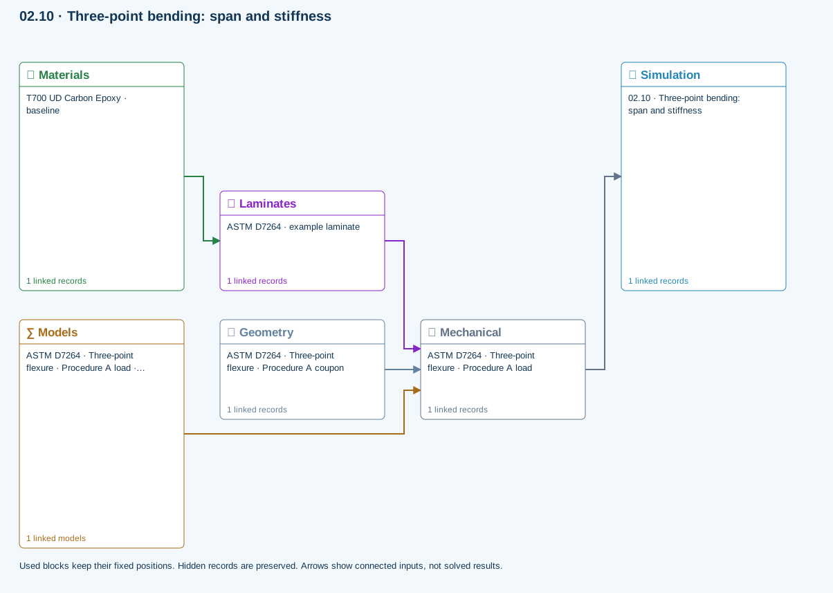
02.10 · Three-point bending: span and stiffness
Level 3IntermediateEst. 25 min
Only blocks on the exercise path are shown. This changes the view only, not the exercise records.
∑ Used models & submodels
Only models assigned to records used by this exercise are listed here. The full-layout option preserves the supplied starter records; no Workbench records are changed.
Euler–Bernoulli beam · Linear static · ASTM D7264 · Three-point flexure · Procedure A load
Beam bending uses effective laminate axial stiffness, the linked section geometry, support span and applied loading. Euler–Bernoulli deflection excludes transverse shear deformation, roller contact and indentation. Ply stress recovery for rectangular laminate coupons is separate from section-level beam stress recovery.
∑ Theory & assumptionsData travelling between blocks
Materials → Laminates
Stored ply stiffness, strength, density and expansion properties.
Mechanical → Simulation
SIMULATION selects this case and its analysis model; the case owns its applicable cycle and input references.
Laminates → Mechanical
Ply angles and thicknesses, stiffness, mass and ply properties.
Geometry → Mechanical
Part shape and dimensions, thickness or section definition, and model-specific geometric inputs. Each selected case consumes only the dimensions its model supports.
Models → Mechanical
Applied model assignment: Euler–Bernoulli beam · Linear static. Model parameters and formulation are used by Mechanical.
Inspect specimen width, laminate thickness, support span and central force.
Models: Euler–Bernoulli beam · ASTM D7264-based
Study scope and limitations
Procedure A teaching setup. Transverse shear deformation, roller contact and indentation are excluded.
Where to find it
In the CLT structural response workspace, open Response → Failure → Fatigue. Run the populated connected simulation first. Supply measured effective-ply fatigue calibration for every active source and stress channel. Fatigue is evaluated separately; the ordinary simulation Run does not evaluate cyclic life automatically.
Upstream coupling
Stored material plies and solved Micro plies use their existing elastic properties, angles and individual thicknesses. The laminate recovers bottom, middle and top ply stresses at two mechanical endpoints. The full six-component Load vector is used at one endpoint and Rload times that vector at the other. Progressive-ramp checkboxes are not fatigue amplitude selectors.
Selected saved thermal, cure and moisture histories contribute fixed residual strain at both endpoints. Available cure-conditioned stiffness is reused through the existing process-state pathway. Changed inputs require a new connected run. The fatigue calibration must independently cover the effective composition, orientation, process state, environment and cycling frequency; elastic homogenization does not create fatigue coefficients.
Model conventions
All stresses are in MPa and N is cycles, not reversals. U is a calibrated curve intercept, not an automatically inferred fiber strength. For peak-based curves, S is the dominant signed endpoint magnitude. Compression-dominated channels reverse sign before forming local R; calibrate with that same convention. Basquin uses half the stress range. No automatic Goodman or other mean-stress correction is applied.
| Model | Implemented relation | Inputs |
|---|---|---|
| Kim–Zhang | N = N₀ + U⁻ᵝ [(S/U)¹⁻ᵝ − 1] / [α(β−1)] | U, α > 0, β > 1, N₀ > 0 |
| Sendeckyj | S = U [1 + C(N−1)]⁻ˢ | U, C > 0, s > 0; controls use α=C and β=s |
| Weibull S–N | S = L + (U−L) exp[−α(log₁₀ N)ᵝ] | U, 0 ≤ L < U, α > 0, β > 0 |
| Kohout–Vechet | S = U [(1 + N/B)/(1 + N/C)]ᵇ | U, 0 < B < C, b < 0 |
| Basquin | Sₐ = A Nᵇ | A > 0, b < 0. Convert reversal-based coefficients before entry. |
The Kim–Zhang stress curve is obtained by algebraically inverting the stated life equation with N−N₀, preserving S=U at N=N₀. Weibull uses log base 10 explicitly: coefficients fitted with natural logarithms must be converted. The Weibull S–N curve is not a probability distribution and supplies no reliability percentile.
Calibration and persistence
- Select the effective ply source, σ1, σ2 or τ12 channel, and dominant sign.
- Select a model and enter its coefficients, published/test source, local stress-ratio bounds and tested cycle range. No material-specific coefficients are prefilled.
- Check that the calibration covers the current composition, process, temperature, moisture and frequency. Confirm applicability; changing inputs resets confirmation.
- Use Store fatigue inputs in CASES, then save the database. The setup follows that case record. Re-run the simulation after storing inputs, then Evaluate fatigue.
Reading results without a false pass
The table reports local endpoint stresses and R, estimated cycles when inside the calibrated domain, and requested cycles divided by estimated life. Missing calibration, zero-amplitude creep-only channels or an endpoint that fails the static ply check are not evaluated. Stresses above the fitted range and lives beyond it are reported separately, with no invented numeric life. Completed does not mean passed; no overall pass is issued, even when requested cycles are below estimated life.
Scope and verification
This is intact, in-plane CLT constant-amplitude screening. It does not update progressive fatigue damage or evolve temperature/cure during cycling. It does not assess delamination growth, adhesive/core fatigue, out-of-plane/FSDT shear, multiaxial fatigue interaction, variable-amplitude accumulation, creep or self-heating. The FSDT, sandwich, joint and layerwise solvers are not replaced by this panel. Frequency is a recorded calibration condition, not a numerical life correction.
Implementation checks cover forward/inverse equations, cycle conventions, monotonicity, numerical stability, thickness/load scaling, fixed residual stresses, missing data, static failure guards and saved-input round trips. These checks are not experimental benchmark validation. No existing teaching material is marked fatigue-qualified by adding this module.
Sources
- Burhan & Kim (2018), S–N Curve Models for Composite Materials Characterisation: equations 8, 11 and 22; model conventions and comparison.
- Sendeckyj (1981), Fitting Models to Composite Materials Fatigue Data: equivalent static strength and fitted fatigue data.
- Kohout & Věchet (2001), A new function for fatigue curves characterization and its multiple merits: full-range curve.
- A generalization of the fatigue Kohout–Věchet model: equivalent parameterizations.
- Kim & Zhang (2001), Fatigue Damage and Life Prediction of Glass/Vinyl Ester Composites: original model study.
- Weibull (1961), Fatigue Testing and Analysis of Results: original fatigue-curve reference.
∑ CLT and residual-strain recovery · ∑ Monotonic progressive failure · ∑ Process coupling
8.4 Specialized constitutive and structural models
06.1 Manuals · read online, preview or download →
Theory / specialized formulations
Mathematical idealizations, constitutive assumptions, calibration requirements and solver limitations.
These studies appear in Workbench → Models → Structural models and in the exercise collection. Each runs separately from coupled process or progressive analyses. Reference-state results are exploratory; analytical software checks do not establish experimentally validated design allowables.
01 · Open-hole strength
Infinite-width, specially orthotropic tension screening. Point and average stress distances must be calibrated independently for this laminate. Not compression, bearing or a joint allowable.
σ(r)/σ∞ = 1 + ½q² + 3/2 q⁴ − ½(Kt − 3)(5q⁶ − 7q⁸), q = a/r.
Constitutive assumptions and calibration
For loading along x, Kt = 1 + √[2(√(Ex/Ey) − νxy) + Ex/Gxy]. The point criterion evaluates stress at a + d₀; the average criterion integrates it from a to a + a₀. Both compare with measured unnotched laminate strength. Their two characteristic lengths need independent calibration. The isotropic limit is Kt = 3.
02 · Creep & stress relaxation
Linear uniaxial response at the calibration temperature. Reference Ex is the instantaneous modulus. Three Maxwell branches; creep is solved from stress equilibrium, not the reciprocal relaxation modulus. No thermal shifting or nonlinear creep.
E(t) = E∞ + Σ Eᵢ exp(−t/τᵢ), E∞ = E₀(1 − Σgᵢ).
Constitutive assumptions and calibration
The laminate reference Ex is E₀. A held-strain experiment gives stress relaxation. For held stress, the solver evolves Maxwell branch stresses and solves equilibrium for strain; creep compliance is not 1/E(t). The calculation compares two time refinements and rejects excessive differences. Three editable branches, one calibration temperature, small uniaxial strain.
03 · Analytical bonded joint
Identical equivalent-elastic adherends, long free arms and a thin elastic adhesive. Compare shear-only Volkersen with eccentric single-lap shear and peel. Not a debonding, plasticity or strength calculation.
Volkersen: τ(x) = (F/b) β cosh(βx) / [2 sinh(βL/2)].
Constitutive assumptions and calibration
β² = 2Ga/(ta Et) for identical adherends. The companion Goland–Reissner solution adds the eccentric-load moment factor and elastic peel distribution. The shared laminate supplies thickness and Ex, with an equivalent-isotropic beam approximation. Adhesive modulus, Poisson ratio, thickness, width and overlap remain explicit study inputs. Peak elastic stress is not a joint-strength prediction.
04 · LaRC04 failure initiation
NASA LaRC04 linear-shear specialization, evaluated at both faces of every ply under membrane and bending loads. Supplied ply strengths are effective/in-situ values; no automatic thin-ply enhancement. Initiation only, not degradation or nonlinear-shear instability.
LaRC04 evaluates matrix tension/compression and fiber tension/kinking in their appropriate fracture and misalignment frames.
Constitutive assumptions and calibration
This release implements the linear-shear specialization of NASA Table 6. CLT recovers stress at both faces of each ply; the kink-frame rotation solves the linear shear equilibrium equation and the fracture-plane search is refined. Supply effective/in-situ strengths explicitly. Identical ply materials share one calibration; mixed-material calibration is rejected. This separate initiation study does not replace or silently extend the progressive-failure solver. Nonlinear-shear instability and delamination are excluded.
05 · Tool-release shape
Free CLT release from prescribed ply-local shrinkage/thermal eigenstrains. Corner spring-in is a separate uniform-strain estimate. Stress-free temperature and effective post-gel shrinkage need calibration. No tool friction, cure kinetics or viscoelastic restraint history.
[ε₀, κ]ᵀ = ABD⁻¹[N*, M*]ᵀ; Δθ = θ(εparallel − εthrough)/(1 + εthrough).
Constitutive assumptions and calibration
The first expression computes free flat-laminate response to prescribed ply-local thermal and post-gel shrinkage strains. The second is a separate uniform-strain corner estimate; positive Δθ means spring-in. The plotted free sections use their center tangent as reference, not a clamp. Enter effective post-gel strains, not total resin volumetric shrinkage. Tool friction, contact and viscoelastic cure history are not resolved.
06 · Fatigue residual properties
Prescribed power-law retention fitted to constant-amplitude tests at a fixed stress ratio, amplitude and temperature. Stiffness and strength have independent coefficients. S–N life alone cannot calibrate either. Does not modify the saved laminate.
E(N)/E₀ = 1 − aE(N/Nf)^bE; X(N)/X₀ = 1 − aX(N/Nf)^bX.
Constitutive assumptions and calibration
This is a prescribed, user-fitted phenomenological retention law. Stiffness and strength use independent loss fractions and exponents. Nf, stress ratio, peak stress and temperature must describe the same constant-amplitude calibration. No extrapolation beyond Nf is allowed. Curves do not automatically modify the saved laminate, and S–N life alone cannot determine degradation coefficients. The reference illustrates why stiffness-degradation data are needed; CDS does not claim to reproduce that NASA fitted model.
07 · Cylinder buckling
Simply supported, thin, specially orthotropic cylinder under uniform axial compression. Discrete Donnell modes; prescribed knockdown factor explores imperfection sensitivity, not a prediction from measured imperfection amplitude. No pressure, torsion, postbuckling or strength pass.
Nx,cr = [D11 k⁴ + 2(D12 + 2D66)k²l² + D22 l⁴ + k⁴/(R²C)] / k².
Constitutive assumptions and calibration
Here k = mπ/L, l = n/R and C = a22k⁴ + (2a12 + a66)k²l² + a11l⁴, with a = A⁻¹. The solver searches discrete axial and circumferential modes for a thin, specially orthotropic simply supported cylinder. A governing mode at the search boundary requires refinement. An explicit knockdown factor scales the ideal result; it is not an automatic prediction from measured imperfections. Pressure, torsion, postbuckling and failure interaction are excluded.
08 · Uncertainty & sensitivity
Seeded independent uniform sampling of shared modulus, ply-thickness and angle offsets. Recomputes laminate ABD for each sample. Bounds are assumptions, not measured distributions. Percentiles and sensitivity are exploratory, not reliability certification.
For each seeded sample: vary bounded inputs → rebuild ABD → solve the axial response.
Constitutive assumptions and calibration
Sampled independent uniform inputs are a common modulus scale, a common thickness scale and a shared ply-angle offset. The output includes strain percentiles and signed Pearson correlations. Repeating the same seed and inputs reproduces the sample set. Zero input ranges recover the deterministic result. Distributions must be justified before drawing reliability conclusions; a small correlation does not rule out nonlinear influence.
Verification before interpretation
Reference checks cover isotropic notch concentration, exact one-branch creep, joint load transfer, pure-load LaRC04 initiation, zero-curvature free expansion, fatigue-retention endpoints, classical isotropic shell buckling and seeded deterministic sampling. Check the scope of each model and repeat sensitivity/convergence studies for your actual inputs. A completed calculation is not an overall design pass.
References
- NASA: notch-strength modelling and characteristic-distance assumptions
- Abaqus: time-domain Prony-series viscoelasticity
- University of Washington: Goland–Reissner calculation equations
- Pinho et al., NASA/TM-2005-213530: original LaRC04 equations
- Analytical modelling of cure-induced laminate deformation
- NASA: measured stiffness degradation for fatigue prognosis
- NASA: shell buckling and imperfection sensitivity
- NASA: uncertainty modelling in composite analysis
8.5 Damage and Failure Framework
Volume III — Damage, Failure, and Software Implementation
Section 1 — Damage and Failure Framework
Executive Summary
This section introduces the damage, failure, and implementation layer of the Workbench micromechanics master model. Volumes I and II define the elastic and thermophysical homogenization framework used to compute effective orthotropic properties for continuous fiber, discontinuous fiber, woven textile, filled matrix, and hybrid composite architectures. Volume III extends the same framework into damage degradation, failure-index evaluation, software data flow, interfaces, and automatic Abaqus material-card export.
The purpose of Section 1 is to define the top-level mathematical and software structure for Volume III. Later sections describe the individual damage models, Tsai-Wu criterion, Hashin criterion, Workbench material properties, and Abaqus export options in greater detail.
1.1 Scope of Volume III
The present volume documents four major capability groups implemented in the solver micromechanics script:
- Continuum damage mechanics (CDM) for stiffness degradation.
- Failure initiation models, including Tsai-Wu and Hashin failure indices.
- composite model, using scalar and vector arrays rather than nested structures or user-defined solver functions.
- Abaqus material-card generation, including engineering constants, transversely isotropic, orthotropic, and fully anisotropic material definitions.
The damage and failure layer is applied after the micromechanics homogenization layer. Therefore, the model can be viewed as a sequential operator chain:
Meaning, notation and theory source
where is the homogenization operator, is the damage operator, is the failure-evaluation operator, and is the export operator used to assemble Workbench and Abaqus outputs.
1.2 Position of Damage and Failure in the Multiscale Workflow
The model first predicts the undamaged effective composite properties. Damage is then applied to the effective stiffness, not to the constituent stiffnesses. This implementation is computationally efficient and appropriate when damage variables are interpreted as homogenized lamina-level state variables.
The undamaged effective stiffness is obtained from the selected micromechanics model:
Meaning, notation and theory source
Definitions and derivation: 1.2 Position of Damage and Failure in the Multiscale Workflow
where is the undamaged effective stiffness tensor. The damaged stiffness is then written as
Meaning, notation and theory source
Definitions and derivation: 1.2 Position of Damage and Failure in the Multiscale Workflow
where is the damage degradation operator. This double-sided form preserves major symmetry of the stiffness matrix and is consistent with common engineering implementations of continuum damage mechanics.
A failure model then evaluates whether the current stress state exceeds an initiation criterion:
Meaning, notation and theory source
Definitions and derivation: 1.2 Position of Damage and Failure in the Multiscale Workflow
where is the failure index, is the stress vector, and denotes the set of strength allowables.
1.3 Damage Variables Used in the solver Model
The implemented damage model uses three scalar damage variables:
Meaning, notation and theory source
Definitions and derivation: 1.3 Damage Variables Used in the solver Model
where is the fiber-direction damage variable, is the matrix/transverse damage variable, and is the shear damage variable. Each variable is bounded as
Meaning, notation and theory source
Definitions and derivation: 1.3 Damage Variables Used in the solver Model
The corresponding damage operator in Voigt notation is
Meaning, notation and theory source
Definitions and derivation: 1.3 Damage Variables Used in the solver Model
The use of a single matrix damage variable for both transverse directions is consistent with the engineering assumption that transverse normal damage is matrix dominated. The shear damage variable is applied to all three shear modes in the simplified composite model.
1.4 Engineering-Constant Form of Damage Degradation
Meaning, notation and theory source
Definitions and derivation: 1.4 Engineering-Constant Form of Damage Degradation
Meaning, notation and theory source
Definitions and derivation: 1.4 Engineering-Constant Form of Damage Degradation
Meaning, notation and theory source
Definitions and derivation: 1.4 Engineering-Constant Form of Damage Degradation
and
Meaning, notation and theory source
Definitions and derivation: 1.4 Engineering-Constant Form of Damage Degradation
where the superscript denotes the undamaged value and denotes the damaged value. These equations summarize the stiffness-degradation logic implemented in the current Workbench-safe solver script.
1.5 Failure Indices and Failure Initiation Logic
The solver script provides two failure-index options: Tsai-Wu and Hashin. The Tsai-Wu failure model is an interactive polynomial criterion for anisotropic materials. In compact form,
Meaning, notation and theory source
Definitions and derivation: 1.5 Failure Indices and Failure Initiation Logic
Failure initiation is predicted when
Meaning, notation and theory source
Definitions and derivation: 1.5 Failure Indices and Failure Initiation Logic
The Hashin model separates fiber and matrix failure modes. The governing Hashin failure index is evaluated as the maximum of the active mode indices:
Meaning, notation and theory source
Definitions and derivation: 1.5 Failure Indices and Failure Initiation Logic
where , , , and denote fiber tension, fiber compression, matrix tension, and matrix compression, respectively.
The failure module is optional. It can be disabled when strength data are unavailable or when the model is used only for property prediction and Abaqus material-card generation.
1.7 Damage and Failure Settings
Table 1 summarizes the damage, failure and export settings.
Table 1. Damage, failure and export settings.
| Setting | Meaning |
|---|---|
| Fiber damage | Fiber-direction continuum damage variable |
| Matrix damage | Matrix/transverse continuum damage variable |
| Shear damage | Shear continuum damage variable |
| Failure model | Selects no failure, Tsai-Wu, Hashin, or both |
| Material export | Enables Abaqus material-card string generation |
| Material definition type | Selects engineering constants, transversely isotropic, orthotropic, or anisotropic card |
The damage variables are interpreted as prescribed state variables. The current script does not automatically evolve damage with load history; rather, it provides the constitutive degradation framework into which an external progressive-damage update law can be inserted later.
1.9 Figure Placeholders
Figure 1. Damage and failure position in the full
micromechanics workflow.
[Insert flowchart showing homogenization, damage degradation, failure
evaluation, property evaluation, and Abaqus export.]
Figure 2. Continuum damage operator acting on the
undamaged effective stiffness matrix.
[Insert schematic showing
,
,
and
.]
1.10 References
- Lemaitre, J. (1996). A Course on Damage Mechanics, 2nd ed. Springer.
- Ladevèze, P. (1983). A damage computational method for composite structures. Computers & Structures.
- Tsai, S. W., and Wu, E. M. (1971). A general theory of strength for anisotropic materials. Journal of Composite Materials, 5, 58-80.
- Hashin, Z. (1980). Failure criteria for unidirectional fiber composites. Journal of Applied Mechanics, 47, 329-334.
- Matzenmiller, A., Lubliner, J., and Taylor, R. L. (1995). A constitutive model for anisotropic damage in fiber-composites. Mechanics of Materials, 20, 125-152.
- Abaqus Documentation. Material definitions: engineering constants, orthotropic elasticity, anisotropic elasticity, expansion, conductivity, and specific heat.
- Jones, R. M. (1999). Mechanics of Composite Materials, 2nd ed. Taylor & Francis.
1.11 Section Summary
Subsequent sections of Volume III document each damage and failure model and then describe the Workbench and Abaqus implementation details in a software-reference format.
8.6 Continuum Damage Mechanics
Volume III — Section 2
Continuum Damage Mechanics and Stiffness Degradation
2.1 Purpose and Scope
The CDM module is not a full progressive failure solver by itself. Instead, it applies user-supplied damage state variables to the effective engineering constants and exports both undamaged and damaged properties. This structure allows Workbench, Abaqus, test correlation scripts, or a future progressive damage law to update the damage variables externally while keeping the micromechanics model stable and transparent.
In the current implementation, the damage variables are:
| Damage variable | solver variable | Physical interpretation |
|---|---|---|
| Fiber-direction damage | Fiber damage | Loss of axial fiber-dominated stiffness |
| Matrix-normal damage | Matrix damage | Loss of transverse matrix-dominated stiffness |
| Shear damage | Shear damage | Loss of shear-transfer stiffness |
2.2 Undamaged Effective Stiffness State
Before damage is applied, the micromechanics branch produces an undamaged orthotropic material state:
Meaning, notation and theory source
Definitions and derivation: 2.2 Undamaged Effective Stiffness State
The corresponding compliance matrix in engineering Voigt notation is:
Meaning, notation and theory source
Definitions and derivation: 2.2 Undamaged Effective Stiffness State
The undamaged stiffness matrix is recovered from:
Meaning, notation and theory source
Definitions and derivation: 2.2 Undamaged Effective Stiffness State
This undamaged state is saved in the solver implementation before degradation so that the output vector can report both pre-damage and post-damage material properties.
2.3 Scalar Damage Variables
The model uses scalar damage variables bounded between zero and unity:
Meaning, notation and theory source
Here, denotes fiber-direction damage, denotes matrix/transverse damage, and denotes shear damage. The limiting values have the following interpretation:
| Value | Meaning |
|---|---|
| Undamaged response | |
| Partially degraded stiffness | |
| Near-complete loss of the associated stiffness mode |
The solver code clips damage values to remain below unity to avoid exactly singular stiffness matrices. This is essential for Workbench and Abaqus workflows, where a zero stiffness can produce ill-conditioned matrices or unstable material cards.
2.4 Damage Operator in Engineering Notation
The implemented damage operator is diagonal in engineering notation:
Meaning, notation and theory source
Definitions and derivation: 2.4 Damage Operator in Engineering Notation
The first component corresponds to the material 1-direction, which is typically the fiber-dominated direction. The second and third components correspond to transverse matrix-dominated normal responses. The final three components correspond to shear responses.
A double-sided damage operation gives the damaged stiffness:
Meaning, notation and theory source
Definitions and derivation: 2.4 Damage Operator in Engineering Notation
The double-sided form preserves the major symmetry of the stiffness matrix:
Meaning, notation and theory source
Definitions and derivation: 2.4 Damage Operator in Engineering Notation
2.5 Engineering-Constant Damage Laws Used in the Code
The implemented stiffness degradation laws are:
Meaning, notation and theory source
Definitions and derivation: 2.5 Engineering-Constant Damage Laws Used in the Code
Meaning, notation and theory source
Definitions and derivation: 2.5 Engineering-Constant Damage Laws Used in the Code
Meaning, notation and theory source
Definitions and derivation: 2.5 Engineering-Constant Damage Laws Used in the Code
Meaning, notation and theory source
Definitions and derivation: 2.5 Engineering-Constant Damage Laws Used in the Code
Meaning, notation and theory source
Definitions and derivation: 2.5 Engineering-Constant Damage Laws Used in the Code
Meaning, notation and theory source
Definitions and derivation: 2.5 Engineering-Constant Damage Laws Used in the Code
The squared form is intentionally conservative relative to a linear knockdown law and reflects the double-sided degradation operator. It also maintains continuity of stiffness as damage evolves.
The Poisson ratios are not explicitly degraded in the current script:
Meaning, notation and theory source
Definitions and derivation: 2.5 Engineering-Constant Damage Laws Used in the Code
This is a practical engineering assumption. In a future extension, Poisson ratios may be recomputed from a fully degraded compliance matrix or linked to damage-mode-specific evolution laws.
2.6 Positive-Definite Stiffness Protection
For numerical robustness, the model applies lower bounds to damaged moduli when the positive-definite projection flag is active. The intent is to ensure:
Meaning, notation and theory source
Definitions and derivation: 2.6 Positive-Definite Stiffness Protection
At the engineering constant level, the stabilized form may be written as:
Meaning, notation and theory source
Definitions and derivation: 2.6 Positive-Definite Stiffness Protection
Meaning, notation and theory source
Definitions and derivation: 2.6 Positive-Definite Stiffness Protection
where and are small positive stiffness floors. This protection prevents singular compliance matrices during Abaqus export and protects the Workbench execution path from divide-by-zero errors.
2.7 Damage and Thermophysical Properties
The current implementation applies CDM only to mechanical stiffness. Effective density, thermal conductivity, coefficient of thermal expansion, and specific heat are computed independently of the damage variables:
Meaning, notation and theory source
Definitions and derivation: 2.7 Damage and Thermophysical Properties
Meaning, notation and theory source
Definitions and derivation: 2.7 Damage and Thermophysical Properties
Meaning, notation and theory source
Definitions and derivation: 2.7 Damage and Thermophysical Properties
Meaning, notation and theory source
Definitions and derivation: 2.7 Damage and Thermophysical Properties
This is appropriate for a first-order engineering material card where damage represents stiffness degradation rather than physical mass loss, crack-surface heat-transfer changes, or evolving thermal expansion. If a coupled thermomechanical damage model is required, thermal conductivity and CTE may be degraded by additional variables or functions of crack density.
2.8 Relationship Between Damage and Failure Criteria
Damage and failure are separate modules in the solver script. Damage modifies the stiffness used to define the exported material response, while failure indices evaluate whether a stress state satisfies a failure criterion. The conceptual workflow is:
Undamaged Micromechanics
        ↓
Effective Engineering Constants
        ↓
Apply Damage Variables
        ↓
Damaged Engineering Constants
        ↓
Evaluate Failure Indices
        ↓
Export Workbench and Abaqus Outputs
The current code uses placeholder stress components unless a future Workbench interface extension supplies applied stress or strain states. The damage module therefore provides stiffness degradation capability independent of stress-driven damage evolution.
2.11 Abaqus Material-Card Implications
When Abaqus export is enabled, the engineering constants written to the material card are the damaged values:
Meaning, notation and theory source
Definitions and derivation: 2.11 Abaqus Material-Card Implications
For *ELASTIC, TYPE=ENGINEERING CONSTANTS, this
produces:
*ELASTIC, TYPE=ENGINEERING CONSTANTS
E1d, E2d, E3d, NU12, NU13, NU23, G12d, G13d, G23d
The Abaqus card is therefore consistent with the damaged stiffness state used by the solver model. The original undamaged properties remain available in the scalar output vector for diagnostics.
2.12 Implementation Notes
- Store undamaged effective stiffness values.
- Clip damage variables to admissible bounds.
- Apply squared degradation factors to and .
- Apply stiffness floors if positive-definite protection is active.
- Export damaged properties to subsequent analysis.
- Use damaged constants in the Abaqus material card.
This structure is robust for Workbench because it avoids nested functions, dynamic objects, and nonlinear iterations inside the damage module.
2.13 Figure Placeholders
Figure 2.1. CDM workflow in the micromechanics
model.
[Insert schematic showing undamaged micromechanics → damage variables →
damaged stiffness → Workbench/Abaqus outputs.]
Figure 2.2. Physical interpretation of
,
,
and
.
[Insert schematic showing axial fiber damage, transverse matrix
cracking, and shear degradation.]
Figure 2.3. Stiffness degradation curves.
[Insert plot of
,
,
and
versus damage variable.]
2.14 References
- Lemaitre, J. (1996). A Course on Damage Mechanics. Springer.
- Kachanov, L. M. (1958). Time of the rupture process under creep conditions. Izvestiya Akademii Nauk SSSR, Otdelenie Tekhnicheskikh Nauk.
- Ladevèze, P. (1983). A damage computational method for composite structures. Computers & Structures.
- Matzenmiller, A., Lubliner, J., and Taylor, R. L. (1995). A constitutive model for anisotropic damage in fiber-composites. Mechanics of Materials.
- Hashin, Z. (1980). Failure criteria for unidirectional fiber composites. Journal of Applied Mechanics.
- Tsai, S. W., and Wu, E. M. (1971). A general theory of strength for anisotropic materials. Journal of Composite Materials.
- Talreja, R. (1985). Transverse cracking and stiffness reduction in composite laminates. Journal of Composite Materials.
- Barbero, E. J. (2018). Finite Element Analysis of Composite Materials Using Abaqus. CRC Press.
8.7 Composite Failure Criteria
Volume III - Section 3
Composite Failure Criteria
3.1 Purpose of the Failure Module
The current implementation supports two classical composite failure formulations:
- Tsai-Wu interactive failure criterion.
- Hashin mode-separated failure criterion.
The purpose of the failure module is not to replace a full progressive damage analysis, but to provide a consistent first-ply or material-point-level failure indicator using the same material property properties carried into the analysis.
| Figure 3.1. Failure evaluation workflow from constituent strengths and material stresses to scalar failure indices. |
Figure 3.1. Failure evaluation workflow from constituent strengths and material stresses to scalar failure indices.
3.2 Stress Components Used by the Failure Model
The failure model is evaluated in the local material coordinate system. The local stress vector is written as
Meaning, notation and theory source
Definitions and derivation: 3.2 Stress Components Used by the Failure Model
where the subscripts 1, 2, and 3 denote the principal orthotropic material directions. Direction 1 is normally associated with the dominant fiber or tow direction, while directions 2 and 3 are matrix-dominated transverse directions.
In the present solver script, the failure stress state is retained as a placeholder stress vector unless external stress inputs are added through Workbench. This design permits the same code framework to be coupled later to structural analysis outputs, coupon-level stress states, or ply-level laminate analysis.
3.3 Strength Inputs
The fiber material property input vector carries the primary tensile, compressive, and shear allowables used by both Tsai-Wu and Hashin models. The strength set is
Meaning, notation and theory source
where
- and are longitudinal tensile and compressive strengths,
- and are transverse tensile and compressive strengths,
- and are third-direction tensile and compressive strengths,
- , , and are shear strengths.
The solver input mapping is summarized in Table 3.1.
Table 3.1. Strength input mapping used by the current solver implementation.
| Input vector index | Symbol | Units | Description |
|---|---|---|---|
| 11 | Pa | Longitudinal tensile strength | |
| 12 | Pa | Longitudinal compressive strength | |
| 13 | Pa | Transverse tensile strength | |
| 14 | Pa | Transverse compressive strength | |
| 15 | Pa | Third-direction tensile strength | |
| 16 | Pa | Third-direction compressive strength | |
| 17 | Pa | 1-2 shear strength | |
| 18 | Pa | 1-3 shear strength | |
| 19 | Pa | 2-3 shear strength |
3.4 Tsai-Wu Failure Criterion
The Tsai-Wu criterion is an interactive polynomial failure theory for anisotropic composite materials. It combines linear stress terms, quadratic stress terms, and interaction terms into a scalar failure index. Failure is predicted when the index reaches unity.
The general form is
Meaning, notation and theory source
with failure initiation defined by
Meaning, notation and theory source
For the three-dimensional orthotropic stress state used in the solver model, the expanded form is
Meaning, notation and theory source
The linear coefficients distinguish tensile and compressive strengths:
Meaning, notation and theory source
The direct quadratic coefficients are
Meaning, notation and theory source
and the shear coefficients are
Meaning, notation and theory source
When biaxial interaction data are unavailable, the implementation uses the common engineering approximation
Meaning, notation and theory source
The Tsai-Wu index is useful when a smooth scalar interaction surface is desired. It is especially convenient for optimization, design-space exploration, and quick screening of material systems.
| Figure 3.2. Schematic Tsai-Wu interaction surface in normal stress space. |
Figure 3.2. Schematic Tsai-Wu interaction surface in normal stress space.
3.5 Hashin Failure Criterion
Hashin failure theory separates failure into physically interpretable fiber and matrix modes. This is useful for composite materials because fiber-dominated and matrix-dominated failures have different consequences for stiffness degradation, residual strength, and progressive damage modeling.
The solver model evaluates four Hashin-type mode indices:
- Fiber tension.
- Fiber compression.
- Matrix tension.
- Matrix compression.
The governing Hashin failure index is the maximum of the active mode indices:
Meaning, notation and theory source
Failure initiation is predicted when
Meaning, notation and theory source
3.6 Fiber Tension Mode
For positive longitudinal stress, the fiber tension index is
Meaning, notation and theory source
This mode represents tensile rupture or tensile-driven degradation of the fiber-dominated direction. In a progressive model, this index would normally be associated with the fiber damage variable .
3.7 Fiber Compression Mode
For negative longitudinal stress, the fiber compression index is implemented as
Meaning, notation and theory source
3.8 Matrix Tension Mode
The matrix tension mode is evaluated when the transverse normal stress sum is tensile:
Meaning, notation and theory source
For , the matrix tension failure index is
Meaning, notation and theory source
Matrix tension is associated with transverse cracking, microcrack initiation, and matrix-dominated stiffness loss.
3.9 Matrix Compression Mode
For , the matrix compression index is implemented as
Meaning, notation and theory source
This form accounts for the interaction between transverse compression and shear loading, which is often critical in matrix-dominated composite failure.
| Figure 3.3. Hashin failure mode map showing fiber tension, fiber compression, matrix tension, and matrix compression regions. |
Figure 3.3. Hashin failure mode map showing fiber tension, fiber compression, matrix tension, and matrix compression regions.
3.10 Failure Model Selection
Choose the failure criterion appropriate to the material and the available strength data.
Table 3.2. Failure model selection logic.
| Active model |
|---|
| No failure calculation |
| Tsai-Wu only |
| Hashin only |
| Tsai-Wu and Hashin |
This flag allows Workbench to activate or deactivate failure calculations without changing the solver script.
3.11 Failure Outputs
The primary scalar outputs from this section are the Tsai-Wu and Hashin failure indices.
Table 3.3. Failure scalar outputs.
| Output index | Variable | Units | Description |
|---|---|---|---|
| 35 | failure_index_tsai_wu |
- | Tsai-Wu failure index |
| 36 | failure_index_hashin |
- | Maximum Hashin failure index |
Model outputs use a consistent metadata convention for downstream reporting.
3.12 Relationship to Damage Variables
The failure criteria compute initiation indices. The continuum damage variables described in Section 2 degrade stiffness:
Meaning, notation and theory source
Definitions and derivation: 3.12 Relationship to Damage Variables
A future progressive failure extension may connect the failure indices to damage update laws of the form
Meaning, notation and theory source
Definitions and derivation: 3.12 Relationship to Damage Variables
Meaning, notation and theory source
Definitions and derivation: 3.12 Relationship to Damage Variables
where may represent cycle count for fatigue extensions, may represent temperature, and is the analysis increment.
The present solver implementation does not automatically evolve damage variables from the failure indices. Instead, damage variables are prescribed through Workbench scalar inputs, while the failure indices provide diagnostic measures.
3.13 Implementation Workflow
The failure calculation sequence is summarized as follows:
Read strength allowables
        |
        v
Read or define local stress state
        |
        v
Compute Tsai-Wu coefficients
        |
        v
Evaluate Tsai-Wu failure index
        |
        v
Evaluate Hashin mode indices
        |
        v
Return scalar failure outputs
This workflow is intentionally simple and deterministic for Workbench execution.
3.14 Applicability and Limitations
The Tsai-Wu model provides a smooth scalar interaction criterion but does not distinguish physical failure modes. Hashin theory provides physically interpretable failure modes but remains an initiation criterion unless coupled to damage evolution laws. Neither criterion alone determines post-failure stiffness evolution. In the current model, stiffness degradation is controlled separately through continuum damage variables.
The failure indices should therefore be interpreted as material-point-level initiation measures and design screening metrics rather than complete progressive failure simulations.
References
- Tsai, S. W., and Wu, E. M. (1971). A general theory of strength for anisotropic materials. Journal of Composite Materials, 5, 58-80.
- Hashin, Z. (1980). Failure criteria for unidirectional fiber composites. Journal of Applied Mechanics, 47, 329-334.
- Hashin, Z., and Rotem, A. (1973). A fatigue failure criterion for fiber reinforced materials. Journal of Composite Materials, 7, 448-464.
- Daniel, I. M., and Ishai, O. (2006). Engineering Mechanics of Composite Materials, 2nd ed. Oxford University Press.
- Jones, R. M. (1999). Mechanics of Composite Materials, 2nd ed. Taylor & Francis.
- Puck, A., and Schurmann, H. (1998). Failure analysis of FRP laminates by means of physically based phenomenological models. Composites Science and Technology, 58, 1045-1067.
- Camanho, P. P., and Matthews, F. L. (1999). A progressive damage model for mechanically fastened joints in composite laminates. Journal of Composite Materials, 33, 2248-2280.
8.8 Damage and Failure Workflow
Volume III – Section 4
Damage and Failure Evaluation Workflow
4.1 Purpose and Scope
The damage and failure workflow is intentionally modular. The effective elastic and thermophysical property predictions can be executed without activating damage or failure. When damage variables are prescribed, the stiffness tensor or engineering constants are degraded before output. When strength allowables and a stress state are available, failure indices are evaluated using the selected criterion. The solver implementation currently supports a prescribed-damage workflow and a failure-index workflow; it does not automatically evolve damage in time unless an external Workbench or solver-level update law supplies new damage variables.
The key workflow outputs are:
- damaged orthotropic engineering constants,
- undamaged reference properties,
- prescribed damage variables,
- Tsai-Wu failure index,
- Hashin modal failure indices,
- maximum governing failure index,
- Abaqus material card data derived from the damaged properties.
4.2 Position of the Damage/Failure Module in the Full Model
The damage and failure module acts after micromechanical homogenization and architecture correction. The full material-property workflow may be summarized as:
Constituent inputs
      -> phase properties
      -> filled matrix / hybrid phase assembly
      -> micromechanics model selection
      -> architecture correction
      -> effective undamaged properties
      -> CDM stiffness degradation
      -> failure index evaluation
      -> effective properties
      -> Abaqus material card string
The model first computes undamaged engineering constants
Meaning, notation and theory source
Definitions and derivation: 4.2 Position of the Damage/Failure Module in the Full Model
After damage degradation, the final output property vector becomes
Meaning, notation and theory source
Definitions and derivation: 4.2 Position of the Damage/Failure Module in the Full Model
In the current engineering implementation, the Poisson ratios are retained from the effective undamaged material state unless a later extension explicitly evolves damage-dependent coupling terms.
4.3 Damage State Vector
The prescribed damage state is represented by three scalar variables:
Meaning, notation and theory source
where is the fiber-direction damage variable, is the matrix-normal damage variable, and is the shear damage variable. Each variable is constrained to the physically meaningful interval
Meaning, notation and theory source
In the solver script, numerical clipping is applied to avoid exactly singular stiffness values:
Meaning, notation and theory source
This rule is not a constitutive law; it is a numerical protection used to maintain finite output properties for Workbench and Abaqus export.
4.4 Engineering-Constant Degradation Workflow
Meaning, notation and theory source
Definitions and derivation: 4.4 Engineering-Constant Degradation Workflow
The transverse moduli are degraded by the matrix-normal damage variable:
Meaning, notation and theory source
Definitions and derivation: 4.4 Engineering-Constant Degradation Workflow
Meaning, notation and theory source
Definitions and derivation: 4.4 Engineering-Constant Degradation Workflow
The shear moduli are degraded by the shear damage variable:
Meaning, notation and theory source
Definitions and derivation: 4.4 Engineering-Constant Degradation Workflow
Meaning, notation and theory source
Definitions and derivation: 4.4 Engineering-Constant Degradation Workflow
Meaning, notation and theory source
Definitions and derivation: 4.4 Engineering-Constant Degradation Workflow
The quadratic degradation form is numerically smooth and ensures monotonic stiffness reduction. It also mirrors the double-sided tensor degradation form introduced in Section 2:
Meaning, notation and theory source
Definitions and derivation: 4.4 Engineering-Constant Degradation Workflow
The direct engineering-constant workflow is preferred in the Workbench script because it avoids user-defined solver functions and avoids repeated tensor assembly for simple engineering studies.
4.5 Positive-Definite Stiffness Protection
After degradation, each modulus is bounded below by a positive floor value:
Meaning, notation and theory source
Definitions and derivation: 4.5 Positive-Definite Stiffness Protection
Meaning, notation and theory source
Definitions and derivation: 4.5 Positive-Definite Stiffness Protection
The floor is not intended to represent real residual material stiffness. It prevents singular compliance matrices when the output is converted into a full stiffness matrix for anisotropic Abaqus export.
The compliance matrix used for orthotropic reconstruction is
Meaning, notation and theory source
Definitions and derivation: 4.5 Positive-Definite Stiffness Protection
The corresponding stiffness matrix is obtained by inversion:
Meaning, notation and theory source
Definitions and derivation: 4.5 Positive-Definite Stiffness Protection
4.6 Failure-Model Selection
Choose the active failure model:
| Failure model |
|---|
| No failure calculation |
| Tsai-Wu only |
| Hashin only |
| Tsai-Wu and Hashin |
The selected failure model is evaluated after the damaged properties have been assembled. The failure model does not modify the stiffness by itself. Instead, it reports failure indices that may be used by Workbench, Abaqus, or an external design loop.
4.7 Stress State for Failure Evaluation
The general three-dimensional stress vector is
Meaning, notation and theory source
Definitions and derivation: 4.7 Stress State for Failure Evaluation
In the current solver implementation, the stress variables are initialized as placeholders unless supplied by a future extension. This design keeps the material-property calculator independent of a structural stress solver. In a coupled workflow, the stress state would be supplied by:
- a laminate analysis tool,
- a finite-element postprocessor,
- a Workbench stress module,
- a load-envelope evaluation routine,
- or a progressive damage loop.
The failure index function can therefore be interpreted as a local material-point assessment operating on the stress vector of Eq. (4.17).
4.8 Tsai-Wu Workflow
When Tsai-Wu is active, the solver computes the scalar failure index
Meaning, notation and theory source
Failure initiation is indicated when
Meaning, notation and theory source
The workflow is:
Read strengths
      -> compute Tsai-Wu coefficients
      -> read stress vector
      -> evaluate quadratic interaction index
      -> report FI_TsaiWu
A design margin may be calculated as
Meaning, notation and theory source
A positive margin indicates that the evaluated stress state is below the Tsai-Wu failure surface.
4.9 Hashin Workflow
When Hashin is active, the model evaluates separate modal indices:
Meaning, notation and theory source
where denotes fiber tension, denotes fiber compression, denotes matrix tension, and denotes matrix compression. Failure initiation is indicated when
Meaning, notation and theory source
The workflow is:
Read strengths
      -> identify stress sign
      -> evaluate fiber mode
      -> evaluate matrix mode
      -> select maximum modal index
      -> report FI_Hashin
Unlike Tsai-Wu, Hashin provides a failure-mode classification. This makes it useful for diagnostic interpretation and progressive damage modeling.
4.10 Governing Failure Status Logic
The implemented failure-status logic is summarized by a governing index:
Meaning, notation and theory source
Definitions and derivation: 4.10 Governing Failure Status Logic
when both criteria are active. A binary failure flag can be defined as
Meaning, notation and theory source
Definitions and derivation: 4.10 Governing Failure Status Logic
The current solver file outputs the indices directly. Workbench can apply Eq. (4.24) externally if a binary pass/fail output is desired.
4.11 Recommended Progressive-Damage Extension
Although the current model uses prescribed damage variables, the same framework can be extended to progressive damage by updating damage as a function of failure index. A simple rate-independent update form is
Meaning, notation and theory source
Definitions and derivation: 4.11 Recommended Progressive-Damage Extension
where
Meaning, notation and theory source
Definitions and derivation: 4.11 Recommended Progressive-Damage Extension
and the Macaulay bracket is
Meaning, notation and theory source
Definitions and derivation: 4.11 Recommended Progressive-Damage Extension
This extension is not required for the present Workbench material-property model, but it provides a clear path for coupling the micromechanics module to nonlinear laminate or finite-element analyses.
4.13 Figure Placeholders
Figure 4.1. Damage and failure workflow.
[Insert flowchart showing homogenization -> damage degradation ->
failure index evaluation -> reported properties -> Abaqus material
card.]
Failure-model selection. Compare Tsai-Wu and Hashin predictions using the same stress state and strength data.
Figure 4.3. Progressive damage extension.
[Insert schematic showing failure index exceeding unity, damage update,
stiffness degradation, and re-evaluation.]
4.14 Implementation Notes
The damage and failure workflow is intentionally kept separate from the homogenization model. This allows the same effective property solver to be used for purely elastic material characterization, damaged-property estimation, or failure-index screening. This separation is also important for Workbench deployment because it avoids state-dependent solver memory unless the user intentionally implements a progressive damage loop outside the script.
- Damage variables are scalar inputs, not hidden internal state variables.
- Failure criteria report indices but do not automatically degrade stiffness.
- Abaqus export uses the final degraded engineering constants.
These rules make the material model deterministic, repeatable, and suitable for automated design studies.
4.15 References
Hashin, Z. (1980). Failure criteria for unidirectional fiber composites. Journal of Applied Mechanics, 47, 329–334.
Ladevèze, P. (1983). A damage mechanics approach for composite materials. Journal of Engineering Materials and Technology, 105, 280–286.
Lemaitre, J. (1996). A Course on Damage Mechanics. Springer.
Matzenmiller, A., Lubliner, J., and Taylor, R. L. (1995). A constitutive model for anisotropic damage in fiber-composites. Mechanics of Materials, 20, 125–152.
Tsai, S. W., and Wu, E. M. (1971). A general theory of strength for anisotropic materials. Journal of Composite Materials, 5, 58–80.
8.9 8. Damage Degradation and Redistribution
8. Damage Degradation and Redistribution
Each ply carries six irreversible stiffness families so the framework can reduce longitudinal, in-plane transverse, through-thickness normal, and three shear responses independently.
Meaning, notation and theory source
Reduces only the longitudinal, transverse, or shear modulus associated with a newly activated failure family.
The rebuilt Qd returns to ABD integration in Eq. 05.3.05-01 at the same load factor.
Definitions and derivation: 8. Damage Degradation and Redistribution
A General-Purpose Hygro-Thermo-Mechanical Progressive-Failure Framework for Continuous and Aligned-Discontinuous Composite Laminates (20 August 2026), source paper supplied for this theory update.
| Failure modes | Primary stiffness | Residual family |
|---|---|---|
| 1–2, fiber tension/compression | E1 | rf |
| 3–4, matrix tension/compression | E2 | rm |
| 5–6, ± in-plane shear | G12 | rs |
| 7–8, through-thickness tension/compression | E3 | rm |
| 9–10, ± local 1–3 shear | G13 | rs |
| 11–12, ± local 2–3 shear | G23 | rs |
Only a newly activated intact family is degraded. Previously failed families do not trigger repeatedly. After each update the reduced stiffness, transformed stiffness, ABD matrix, environmental resultants, generalized strains, and all ply stresses are rebuilt, allowing load redistribution to expose secondary failures.
Event identity
Every event stores load step, pseudo-time/load factor, ply number, top or bottom surface, signed failure mode, index value, material type, selected criterion, local stress vector, and through-thickness coordinate.
8.10 10. Mixed-Mode Cohesive Delamination
10. Mixed-Mode Cohesive Delamination
The optional interface branch uses a bilinear irreversible cohesive law with quadratic initiation and Benzeggagh–Kenane mixed-mode propagation.
Meaning, notation and theory source
Maps positive normal and two shear separations to interface trial tractions.
Supplies the tractions evaluated by the initiation surface in Eq. 05.3.10-02.
Definitions and derivation: 10. Mixed-Mode Cohesive Delamination
A General-Purpose Hygro-Thermo-Mechanical Progressive-Failure Framework for Continuous and Aligned-Discontinuous Composite Laminates (20 August 2026), source paper supplied for this theory update.
Meaning, notation and theory source
Triggers cohesive damage when the combined normalized traction reaches one.
After initiation, mixed-mode fracture energy is determined by Eq. 05.3.10-03.
Definitions and derivation: 10. Mixed-Mode Cohesive Delamination
A General-Purpose Hygro-Thermo-Mechanical Progressive-Failure Framework for Continuous and Aligned-Discontinuous Composite Laminates (20 August 2026), source paper supplied for this theory update.
Meaning, notation and theory source
Interpolates critical fracture energy from the shear fraction of total energy release.
Gc determines the terminal separation used by Eq. 05.3.10-04.
Definitions and derivation: 10. Mixed-Mode Cohesive Delamination
A General-Purpose Hygro-Thermo-Mechanical Progressive-Failure Framework for Continuous and Aligned-Discontinuous Composite Laminates (20 August 2026), source paper supplied for this theory update.
Meaning, notation and theory source
Evolves interface damage from initiation separation to complete decohesion.
The maximum interface damage may feed the reduced-order bending-stiffness update described below.
Definitions and derivation: 10. Mixed-Mode Cohesive Delamination
A General-Purpose Hygro-Thermo-Mechanical Progressive-Failure Framework for Continuous and Aligned-Discontinuous Composite Laminates (20 August 2026), source paper supplied for this theory update.
Tensile and shear tractions are multiplied by (1−d); compression remains elastic. A reduced-order laminate feedback may use Deff=(1−dmax)Dintact+dmaxDsplit, while Aeff=Aintact.
Chapter review
Compare the model against appropriate independent tests and state the loading and geometry domain of that comparison. Agreement with a single case is not a general validation claim. Numerical checks, parameter fitting and experimental validation serve different purposes.
References and source sections
References are retained with the formulations they support. Software instructions describe implementation scope; a cited source does not establish independent validation of a CDS calculation.
- Soden, P. D., Hinton, M. J., and Kaddour, A. S. (1998). A comparison of the predictive capabilities of current failure theories for composite laminates. Composites Science and Technology, 58, 1225–1254.
- Tsai, S. W., and Wu, E. M. (1971). A General Theory of Strength for Anisotropic Materials. Journal of Composite Materials, 5(1), 58–80.
- Hashin, Z. (1980). Failure Criteria for Unidirectional Fiber Composites. Journal of Applied Mechanics, 47(2), 329–334.
- Burhan & Kim (2018), S–N Curve Models for Composite Materials Characterisation
- Sendeckyj (1981), Fitting Models to Composite Materials Fatigue Data
- Kohout & Věchet (2001), A new function for fatigue curves characterization and its multiple merits
- A generalization of the fatigue Kohout–Věchet model
- Kim & Zhang (2001), Fatigue Damage and Life Prediction of Glass/Vinyl Ester Composites
- Weibull (1961), Fatigue Testing and Analysis of Results
- NASA: notch-strength modelling and characteristic-distance assumptions
- Abaqus: time-domain Prony-series viscoelasticity
- University of Washington: Goland–Reissner calculation equations
- Pinho et al., NASA/TM-2005-213530: original LaRC04 equations
- Analytical modelling of cure-induced laminate deformation
- NASA: measured stiffness degradation for fatigue prognosis
- NASA: shell buckling and imperfection sensitivity
- NASA: uncertainty modelling in composite analysis
- Camanho, P. P., and Dávila, C. G. (2002). Mixed-Mode Decohesion Finite Elements for the Simulation of Delamination in Composite Materials. NASA/TM-2002-211737.
- Turon, A., Camanho, P. P., Costa, J., and Dávila, C. G. (2006). A damage model for the simulation of delamination in advanced composites under variable-mode loading. Mechanics of Materials, 38, 1072–1089.
- Benzeggagh, M. L., and Kenane, M. (1996). Measurement of mixed-mode delamination fracture toughness of unidirectional glass/epoxy composites with mixed-mode bending apparatus. Composites Science and Technology, 56, 439–449.