
Micromechanics maps constituent properties and architecture to an effective ply. The calculation requires a representative reinforcement arrangement and volume fractions. It does not replace measured design allowables or establish that a manufactured material has the assumed architecture.
Mixture estimates, inclusion models and shear-lag models make different assumptions about load transfer, geometry and interaction. Continuous aligned fibers, short fibers, fabrics and particle-filled systems require different architecture descriptions. Verify constituent limits and the effect of orientation and aspect ratio before comparing a predicted effective modulus with a test.
Pass the effective elastic tensor, density and directional expansion and transport properties with their coordinate convention. Retain separate provenance for each property family. A model calibrated for elastic stiffness is not automatically calibrated for thermal conductivity, diffusion or strength.
3.1 Micromechanics of Composites
Current Workbench models and compatibility
This theory library includes wider research formulations. Check the released model directory for selectable models, required inputs, limits and exercises. The event-driven RVE branch is not enabled in hosted Workbench.
Theories / Micromechanics
The complete CDS theory chain: continuous and discontinuous fibers, mean-field homogenization, Chou orientation factors, textile architectures, fillers and voids, thermophysics, damage and failure, constituent-limit recovery, and the per-ply handoff into progressive laminate analysis.
Theory map
Models, equations, figures, and cross-referencesConstituent to effective stiffness
Continuous and discontinuous fibers; rule of mixtures, Halpin–Tsai, Mori–Tanaka, self-consistent formulations; aspect ratio; global orientation; Chou Fa/Fp; constituent-limit recovery; compliance and stiffness matrices.
Open elastic theory →Random ends, Weibull strengths, and critical clusters
This reference describes the Henry–Pimenta event-driven RVE formulation. It is not enabled in hosted Workbench; the released Cox elastic short-fiber model has a narrower supported scope.
Open discontinuous-fiber theory →Tows, fabrics, and architecture corrections
Plain weave, 2×2 twill, 4/5/8-harness satin, basket, leno, biaxial NCF, and triaxial braid with warp–weft averaging, crimp, interlacing, stitch, binder, and bias-angle effects.
Open fabric theory →Fillers, voids, and thermophysical response
Filled-resin and hybrid homogenization, explicit and dilute directional void treatment, density, specific heat, orthotropic conductivity, directional CTE, validation checks, and linked references.
Open filler and void theory →CDM and composite failure
Continuum damage mechanics, Tsai–Wu and Hashin criteria, recovered endpoint properties, degradation, and failure progression.
Open failure theory →Generated properties enter progressive laminates
Each physical ply independently selects automatic property resolution, embedded constituent micromechanics, or direct measured data. The generated pristine 3D property set then enters the common damaged-ABD and failure-redistribution solver.
Open unified material routing →Complete reference
One continuous sequenceElastic Micromechanics Theory
→02Aligned Discontinuous-Fiber Model
→03Textile and Thermophysical Framework
→04Fabric Micromechanics Theory
→05Warp–Weft Averaging and Crimp Correction
→06Filled Matrix, Hybrid, and Void Micromechanics
→07Effective Density and Specific Heat
→08Thermal Conductivity Micromechanics
→09CTE Micromechanics
→10Orthotropic Thermophysical Property Assembly
→11Verification, Validation, and References
→12Damage and Failure Framework
→13Continuum Damage Mechanics
→14Composite Failure Criteria
→15Damage and Failure Workflow
→3.2 Elastic Micromechanics Theory
Table of Contents
1 Preface
2 Abstract
A compact elastic micromechanics framework is described for predicting the effective orthotropic stiffness of continuous fiber, discontinuous fiber, woven, filler-reinforced, and general multiphase composite materials. The model permits selection among four main homogenization branches: rule of mixtures, Halpin–Tsai, Mori–Tanaka engineering approximation, and a self-consistent engineering approximation. Constituent properties are supplied through Workbench vector inputs, while microstructure descriptors are supplied through scalar flags and scalar parameters. Fiber architecture effects are represented using fiber volume fraction, aspect ratio, and Tsu-Wei Chou axial and planar architecture parameters, denoted and . The model outputs effective Young’s moduli, shear moduli, Poisson ratios, and related quantities for use in subsequent laminate and structural studies.
3 Nomenclature
| Symbol | Definition | Units |
|---|---|---|
| Effective orthotropic Young’s moduli | Pa | |
| Effective orthotropic shear moduli | Pa | |
| Effective major Poisson ratios | – | |
| Fiber, matrix, particle/filler, and void volume fractions | – | |
| Fiber, matrix, and particle moduli | Pa | |
| Fiber, matrix, and particle shear moduli | Pa | |
| Fiber or inclusion aspect ratio, usually | – | |
| Fiber length efficiency factor | – | |
| Orientation efficiency factor | – | |
| Chou axial architecture factor | – | |
| Chou planar/random architecture factor | – | |
| Halpin–Tsai shape parameter | – | |
| Halpin–Tsai contrast parameter | – | |
| Stiffness matrix or fourth-order stiffness tensor | Pa | |
| Compliance matrix or Eshelby tensor depending on context | or – | |
| Strain concentration tensor or matrix | – | |
| Macroscopic stress | Pa | |
| Macroscopic strain | – | |
| Global material orientation angle | deg |
4 1. Model Scope
The solver model predicts effective properties of composite materials from constituent properties and architecture descriptors. The main elastic outputs are the orthotropic engineering constants
Meaning, notation and theory source
These properties are used to generate Abaqus material definitions. Choose from the following stiffness models:
| Model branch |
|---|
| Rule of mixtures |
| Halpin–Tsai |
| Mori–Tanaka engineering approximation |
| Self-consistent engineering approximation |
Choose the material architecture independently of the stiffness model:
| Architecture branch |
|---|
| Continuous unidirectional fiber composite |
| Discontinuous fiber composite |
| Woven fabric composite |
| General multiphase composite |
This separation allows, for example, a discontinuous-fiber material to be evaluated using a simple rule-of-mixtures approximation or a more interaction-aware self-consistent approximation.
5 2. Constituent Property Inputs
Specify the properties of each constituent. The fiber property vector contains anisotropic stiffnesses, strengths, density, and thermophysical values. In Volume I only the elastic terms are required:
Meaning, notation and theory source
Definitions and derivation: 5 2. Constituent Property Inputs
The matrix vector contains isotropic elastic properties,
Meaning, notation and theory source
Definitions and derivation: 5 2. Constituent Property Inputs
and the filler vector contains particle properties,
Meaning, notation and theory source
Definitions and derivation: 5 2. Constituent Property Inputs
The matrix shear modulus is computed from isotropic elasticity:
Meaning, notation and theory source
Definitions and derivation: 5 2. Constituent Property Inputs
Similarly, for an isotropic particle phase,
Meaning, notation and theory source
Definitions and derivation: 5 2. Constituent Property Inputs
6 3. Constituent Stiffness and Compliance
Meaning, notation and theory source
Definitions and derivation: 6 3. Constituent Stiffness and Compliance
where denotes the phase. For an isotropic phase, the stiffness tensor is
Meaning, notation and theory source
Definitions and derivation: 6 3. Constituent Stiffness and Compliance
with
Meaning, notation and theory source
Definitions and derivation: 6 3. Constituent Stiffness and Compliance
For an orthotropic fiber, the compliance matrix in material coordinates is conventionally written as
Meaning, notation and theory source
Definitions and derivation: 6 3. Constituent Stiffness and Compliance
The reciprocal Poisson ratios satisfy
Meaning, notation and theory source
Definitions and derivation: 6 3. Constituent Stiffness and Compliance
The stiffness matrix is obtained by inversion:
Meaning, notation and theory source
Definitions and derivation: 6 3. Constituent Stiffness and Compliance
7 4. Volume Fractions and Phase Normalization
The model normalizes phase volume fractions so that
Meaning, notation and theory source
Definitions and derivation: 7 4. Volume Fractions and Phase Normalization
where is the optional void volume fraction. If the filler is treated implicitly, the matrix is first modified and the explicit particle phase is set to zero. If the filler is treated explicitly, the global particle fraction is estimated from the filler fraction inside the resin phase:
Meaning, notation and theory source
Definitions and derivation: 7 4. Volume Fractions and Phase Normalization
The remaining matrix fraction is then
Meaning, notation and theory source
Definitions and derivation: 7 4. Volume Fractions and Phase Normalization
This normalization is important because all mixture and mean-field equations assume that the phase fractions sum to unity.
8 5. Implicit Filled Matrix Model
Before fiber/matrix homogenization, a filler can be used to modify the matrix modulus. The current script uses a Halpin–Tsai style spherical-particle correction. The effective filled matrix modulus is
Meaning, notation and theory source
Definitions and derivation: 8 5. Implicit Filled Matrix Model
where
Meaning, notation and theory source
Definitions and derivation: 8 5. Implicit Filled Matrix Model
The filled matrix shear modulus is
Meaning, notation and theory source
Definitions and derivation: 8 5. Implicit Filled Matrix Model
with
Meaning, notation and theory source
Definitions and derivation: 8 5. Implicit Filled Matrix Model
A consistent effective Poisson ratio is recovered by
Meaning, notation and theory source
Definitions and derivation: 8 5. Implicit Filled Matrix Model
This option is computationally efficient and appropriate when filler is treated as a matrix modifier rather than as a separate interacting phase.
9 6. Rule of Mixtures
The rule-of-mixtures model is the simplest model and is retained as a bounding and verification option. In the fiber direction, the iso-strain assumption gives
Meaning, notation and theory source
The phase-averaged stress is
Meaning, notation and theory source
Substituting phase constitutive laws yields the Voigt axial modulus
Meaning, notation and theory source
For transverse loading, the inverse or Reuss estimate is used:
Meaning, notation and theory source
Similarly,
Meaning, notation and theory source
The shear moduli are estimated using inverse mixtures:
Meaning, notation and theory source
Meaning, notation and theory source
and
Meaning, notation and theory source
The major Poisson ratios are computed by direct mixture:
Meaning, notation and theory source
The same form is used for and . The rule-of-mixtures option is not intended to capture inclusion interaction, but it provides a transparent reference case and useful numerical sanity check.
10 7. Halpin–Tsai Model
The Halpin–Tsai model provides a semi-empirical correction for reinforcement geometry and phase contrast. For a generic engineering modulus , the Halpin–Tsai form is
Meaning, notation and theory source
where
Meaning, notation and theory source
For transverse Young’s modulus, the code uses the common circular-fiber estimate
Meaning, notation and theory source
so that
Meaning, notation and theory source
with
Meaning, notation and theory source
The third-direction modulus is treated analogously:
Meaning, notation and theory source
The shear moduli are estimated using
Meaning, notation and theory source
where
Meaning, notation and theory source
The code uses as a default engineering estimate. The same equation form is applied to and . Halpin–Tsai is more physically representative than rule of mixtures for transverse and shear properties, but the parameter is empirical and should be calibrated when reliable data are available.
11 8. Mori–Tanaka Mean-Field Theory
The classical Mori–Tanaka method is based on an inclusion phase embedded in a matrix reference medium. In compact tensor notation, the inclusion strain concentration tensor is
Meaning, notation and theory source
Definitions and derivation: 11 8. Mori–Tanaka Mean-Field Theory
where is the Eshelby tensor. The Mori–Tanaka stiffness is commonly written as
Meaning, notation and theory source
Definitions and derivation: 11 8. Mori–Tanaka Mean-Field Theory
For multiple inclusion phases, a normalized mean-field form may be written as
Meaning, notation and theory source
Definitions and derivation: 11 8. Mori–Tanaka Mean-Field Theory
Meaning, notation and theory source
Definitions and derivation: 11 8. Mori–Tanaka Mean-Field Theory
where is an interaction factor depending on and stiffness contrast. The implemented form is an engineering approximation to the interaction behavior of a mean-field model:
Meaning, notation and theory source
Definitions and derivation: 11 8. Mori–Tanaka Mean-Field Theory
The transverse and shear terms are based on Halpin–Tsai values with a small aspect-ratio-dependent correction. The aspect ratio factor is
Meaning, notation and theory source
Definitions and derivation: 11 8. Mori–Tanaka Mean-Field Theory
A representative transverse correction is
Meaning, notation and theory source
Definitions and derivation: 11 8. Mori–Tanaka Mean-Field Theory
The Mori–Tanaka option should therefore be interpreted as a computationally robust engineering approximation to mean-field behavior rather than a complete fourth-order tensor Mori–Tanaka implementation.
12 9. Self-Consistent Field Theory and Implemented Approximation
In the full self-consistent theory, each phase is embedded in the unknown effective medium instead of in the matrix. The governing consistency equation is
Meaning, notation and theory source
Definitions and derivation: 12 9. Self-Consistent Field Theory and Implemented Approximation
The phase concentration tensor is
Meaning, notation and theory source
Definitions and derivation: 12 9. Self-Consistent Field Theory and Implemented Approximation
A fixed-point update form is
Meaning, notation and theory source
Definitions and derivation: 12 9. Self-Consistent Field Theory and Implemented Approximation
Meaning, notation and theory source
Definitions and derivation: 12 9. Self-Consistent Field Theory and Implemented Approximation
with
Meaning, notation and theory source
Definitions and derivation: 12 9. Self-Consistent Field Theory and Implemented Approximation
The transverse moduli are blended from Halpin–Tsai and a stiffness-interaction term:
Meaning, notation and theory source
Definitions and derivation: 12 9. Self-Consistent Field Theory and Implemented Approximation
Meaning, notation and theory source
Definitions and derivation: 12 9. Self-Consistent Field Theory and Implemented Approximation
The shear moduli use analogous blended expressions:
Meaning, notation and theory source
Definitions and derivation: 12 9. Self-Consistent Field Theory and Implemented Approximation
and similarly for . This form is designed to remain stable in Workbench while providing a stronger interaction correction than the pure Halpin–Tsai model.
13 10. Continuous Fiber Composite Model
For continuous fibers, the length efficiency is set to unity:
Meaning, notation and theory source
Definitions and derivation: 13 10. Continuous Fiber Composite Model
The axial orientation factor is forced close to the aligned limit:
Meaning, notation and theory source
Definitions and derivation: 13 10. Continuous Fiber Composite Model
For continuous aligned fibers, the axial modulus approaches the Voigt expression
Meaning, notation and theory source
Definitions and derivation: 13 10. Continuous Fiber Composite Model
However, the transverse and shear properties are still computed from the selected micromechanics branch. This distinction is important: even when the axial response is mixture-like, the transverse stiffness and shear stiffness remain controlled by matrix constraint, fiber packing, and phase interaction. The continuous fiber branch is appropriate for unidirectional prepreg laminae, pultruded rods, filament-wound laminae, and tow-level properties in woven fabrics.
14 11. Discontinuous Fiber Composite Model
Model scope. This section describes the compact elastic architecture-efficiency path. The unified solver's criterion-6 tensile branch implements the complete Henry and Pimenta (2017) event-driven workflow: reconstructed broken/shear-lag interaction segments, a generic nonlinear matrix shear law, ordered Weibull breaks, same-strain network rebuilding, RVE series coupling, pull-out resistance, and nonlinear critical-cluster termination. See the aligned discontinuous-fiber theory and traceability page.
In short-fiber composites, a fiber does not generally reach the full far-field axial stress because stress must build up through matrix-to-fiber shear transfer. The model uses a compact length efficiency factor
Meaning, notation and theory source
Definitions and derivation: 14 11. Discontinuous Fiber Composite Model
where
Meaning, notation and theory source
Definitions and derivation: 14 11. Discontinuous Fiber Composite Model
This expression has the correct limits:
Meaning, notation and theory source
Definitions and derivation: 14 11. Discontinuous Fiber Composite Model
and
Meaning, notation and theory source
Definitions and derivation: 14 11. Discontinuous Fiber Composite Model
The axial contribution of short fibers is then reduced by length and orientation factors:
Meaning, notation and theory source
Definitions and derivation: 14 11. Discontinuous Fiber Composite Model
The implemented code uses the Chou axial factor as the default orientation efficiency:
Meaning, notation and theory source
Definitions and derivation: 14 11. Discontinuous Fiber Composite Model
The transverse moduli are modified by a planar/random architecture correction. A representative engineering correction is
Meaning, notation and theory source
Definitions and derivation: 14 11. Discontinuous Fiber Composite Model
with a similar expression for . This correction reduces directional stiffness when fibers are less aligned and redistributes stiffness into planar directions as the random component increases.
15 12. Tsu-Wei Chou Architecture Factors
The model uses compact Chou-style architecture parameters to describe orientation effects without requiring the Workbench user to enter a full orientation tensor. The axial parameter represents the fourth-order projection of fiber direction onto the primary material axis:
Meaning, notation and theory source
Definitions and derivation: 15 12. Tsu-Wei Chou Architecture Factors
The planar or random contribution is represented as
Meaning, notation and theory source
Definitions and derivation: 15 12. Tsu-Wei Chou Architecture Factors
or as an independently supplied parameter when calibrated from data. The axial stiffness contribution is governed primarily by :
Meaning, notation and theory source
Definitions and derivation: 15 12. Tsu-Wei Chou Architecture Factors
A compact architecture-modified stiffness expression is
Meaning, notation and theory source
Definitions and derivation: 15 12. Tsu-Wei Chou Architecture Factors
For a perfectly aligned material,
Meaning, notation and theory source
Definitions and derivation: 15 12. Tsu-Wei Chou Architecture Factors
For planar random orientation, is smaller and is larger. For three-dimensional random orientation, the axial fourth-order projection is lower still. The representation is less general than a full second- and fourth-order orientation tensor, but it is much more compact and well suited for Workbench front-panel entry.
16 13. Orthotropic Engineering Constant Extraction
After the selected micromechanics branch and architecture corrections are applied, the model assembles effective engineering constants. The major Poisson ratios are estimated by direct mixture:
Meaning, notation and theory source
Definitions and derivation: 16 13. Orthotropic Engineering Constant Extraction
Meaning, notation and theory source
Definitions and derivation: 16 13. Orthotropic Engineering Constant Extraction
Meaning, notation and theory source
Definitions and derivation: 16 13. Orthotropic Engineering Constant Extraction
The effective compliance matrix is then assembled as
Meaning, notation and theory source
Definitions and derivation: 16 13. Orthotropic Engineering Constant Extraction
The stiffness matrix used for anisotropic Abaqus export is
Meaning, notation and theory source
Definitions and derivation: 16 13. Orthotropic Engineering Constant Extraction
When the positive-definite projection flag is enabled, the model applies lower bounds to moduli and regularizes ill-conditioned matrices to prevent nonphysical Abaqus material definitions.
17 14. Workflow Summary
- Parse material and architecture flags.
- Construct matrix, fiber, filler, and void phase properties.
- Apply implicit filled-matrix correction if required.
- Normalize all phase volume fractions.
- Choose the micromechanics model.
- Choose the material architecture.
- Compute baseline elastic constants.
- Apply discontinuous-fiber, Chou, or woven architecture corrections.
- Compute Poisson ratios and assemble the compliance matrix.
- Pass the dense property state through the thermophysical, void, damage, and failure branches documented in Volumes II and III.
- Apply the global constituent-limit recovery check to the final property state.
- Rebuild compliance, stiffness, finite-element properties, and material exports from the recovered state.
- Store results in Workbench scalar, vector, matrix, and selected-string outputs.
18 15. Constituent-Limit Recovery
Every homogenization branch is required to recover the exact active constituent at a pure-phase endpoint. This is an implementation verification condition as well as a physical consistency condition. If phase is dominant within the selected tolerance, the final mechanical and thermophysical property vector is replaced by that phase vector:
Meaning, notation and theory source
Definitions and derivation: 18 15. Constituent-Limit Recovery
The recovered vector includes the elastic constants, density, specific heat, directional conductivity, and directional CTE. Thus returns the fiber properties exactly; matrix- and filler-dominated limits recover their corresponding phase definitions. The void endpoint uses the defined void state.
Recovery is deliberately applied after homogenization, architecture, thermophysical, void, and damage/failure operations. Every dependent quantity is then regenerated: orthotropic and anisotropic stiffness and compliance matrices, effective properties, scalar diagnostics, Workbench FE matrices, and the selected material export. This ordering prevents a later correction from overwriting the endpoint state or an export from retaining stale pre-recovery values. See and .
19 16. Applicability and Limitations
The current implementation is most appropriate for preliminary design, material screening, embedded Workbench workflows, and automated Abaqus material-card generation. It is not intended to replace detailed finite-element RVE homogenization when exact tow geometry, interphase behavior, nonlinear matrix response, or progressive damage evolution must be resolved explicitly.
20 References
Advani, S. G., and Tucker, C. L. III (1987). The use of tensors to describe and predict fiber orientation in short fiber composites. Journal of Rheology, 31, 751–784.
Benveniste, Y. (1987). A new approach to the application of Mori–Tanaka’s theory in composite materials. Mechanics of Materials, 6, 147–157.
Budiansky, B. (1965). On the elastic moduli of some heterogeneous materials. Journal of the Mechanics and Physics of Solids, 13, 223–227.
Chou, T.-W., Nomura, S., and Taya, M. (1980). A self-consistent approach to the elastic stiffness of short-fiber composites. Journal of Composite Materials, 14, 178–188.
Christensen, R. M. (1979). Mechanics of Composite Materials. Wiley.
Cox, H. L. (1952). The elasticity and strength of paper and other fibrous materials. British Journal of Applied Physics, 3, 72–79.
Henry, J., and Pimenta, S. (2017). Semi-analytical simulation of aligned discontinuous composites. Composites Science and Technology, 144, 230–244. doi:10.1016/j.compscitech.2017.01.027.
Eshelby, J. D. (1957). The determination of the elastic field of an ellipsoidal inclusion, and related problems. Proceedings of the Royal Society of London A, 241, 376–396.
Folgar, F., and Tucker, C. L. III (1984). Orientation behavior of fibers in concentrated suspensions. Journal of Reinforced Plastics and Composites, 3, 98–119.
Halpin, J. C., and Kardos, J. L. (1976). The Halpin–Tsai equations: A review. Polymer Engineering and Science, 16, 344–352.
Hill, R. (1965). A self-consistent mechanics of composite materials. Journal of the Mechanics and Physics of Solids, 13, 213–222.
Jones, R. M. (1999). Mechanics of Composite Materials, 2nd ed. Taylor & Francis.
Mori, T., and Tanaka, K. (1973). Average stress in matrix and average elastic energy of materials with misfitting inclusions. Acta Metallurgica, 21, 571–574.
Mura, T. (1987). Micromechanics of Defects in Solids, 2nd ed. Martinus Nijhoff.
Nemat-Nasser, S., and Hori, M. (1999). Micromechanics: Overall Properties of Heterogeneous Materials, 2nd ed. Elsevier.
Tandon, G. P., and Weng, G. J. (1984). The effect of aspect ratio of inclusions on the elastic properties of unidirectionally aligned composites. Polymer Composites, 5, 327–333.
3.3 Thermal Conductivity Micromechanics
Volume II - Section 6: Thermal Conductivity Micromechanics
6.1 Purpose and Scope
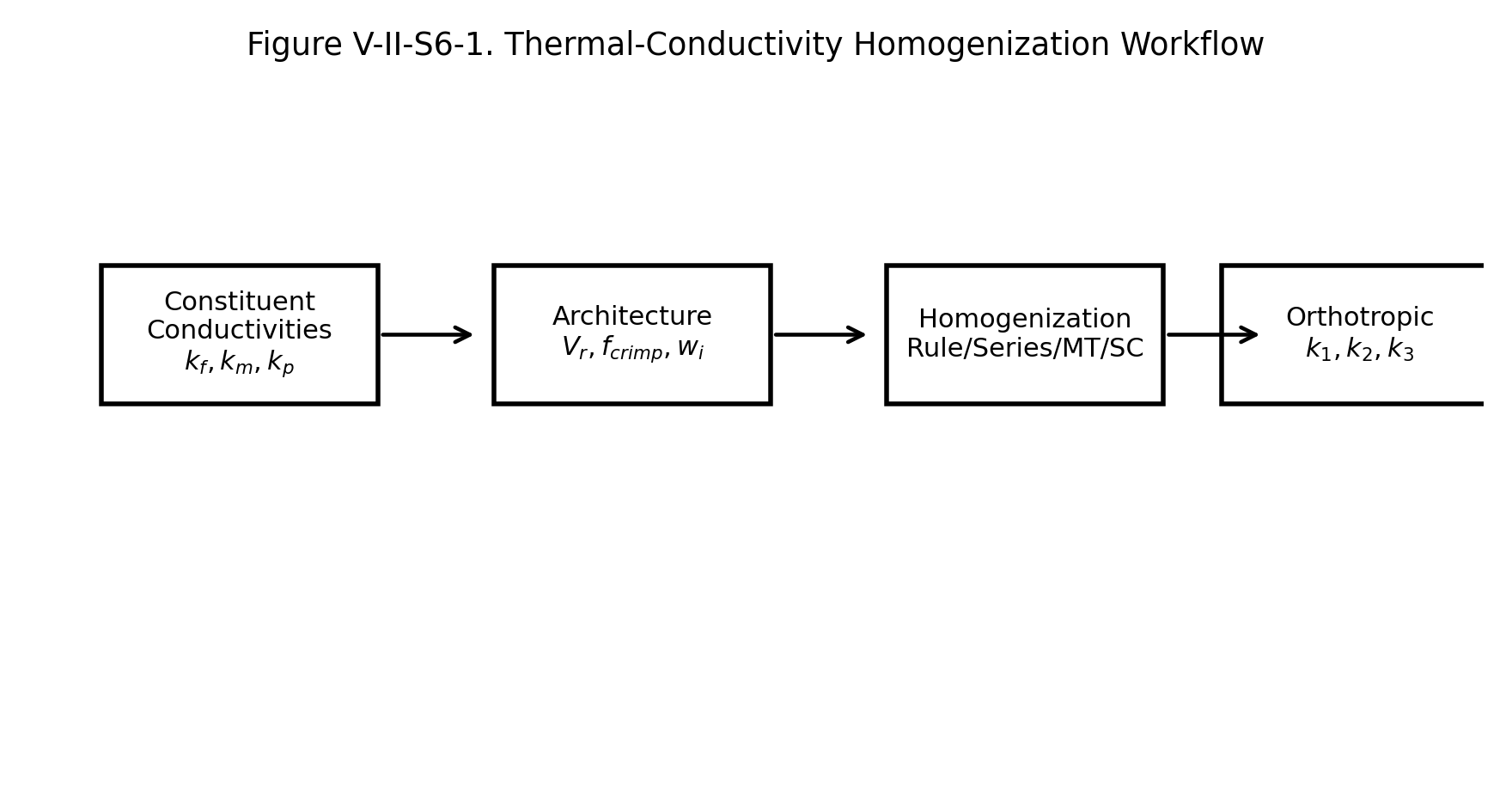
Figure V-II-S6-1. Thermal-conductivity homogenization workflow used by the Workbench micromechanics implementation.
6.2 Local Heat-Conduction Law
The local thermal field is assumed to satisfy Fourier’s law in each phase,
Meaning, notation and theory source
where is the phase heat flux vector, is the phase thermal conductivity tensor, and is the local temperature field. For an effective homogeneous composite, the corresponding macroscopic relation is
Meaning, notation and theory source
For an orthotropic material aligned with the material principal axes, the conductivity tensor is diagonal,
Meaning, notation and theory source
The solver implementation outputs the three principal components , , and because these are the values required by Abaqus for an orthotropic conductivity card.
6.3 Rule-of-Mixtures Conductivity Limits
For heat flow parallel to continuous fibers or aligned high-conductivity inclusions, the Voigt-type expression is used,
Meaning, notation and theory source
Definitions and derivation: 6.3 Rule-of-Mixtures Conductivity Limits
For heat flow normal to layered or fiber-like phase paths, the Reuss-type series expression is
Meaning, notation and theory source
Definitions and derivation: 6.3 Rule-of-Mixtures Conductivity Limits
For a fiber-matrix-filler-void system, the implemented parallel idealization is
Meaning, notation and theory source
Definitions and derivation: 6.3 Rule-of-Mixtures Conductivity Limits
The transverse or through-thickness conductivity may be estimated as
Meaning, notation and theory source
Definitions and derivation: 6.3 Rule-of-Mixtures Conductivity Limits
and
Meaning, notation and theory source
Definitions and derivation: 6.3 Rule-of-Mixtures Conductivity Limits
In the numerical implementation, the void conductivity is assigned a small positive value rather than zero so that division by zero is avoided.
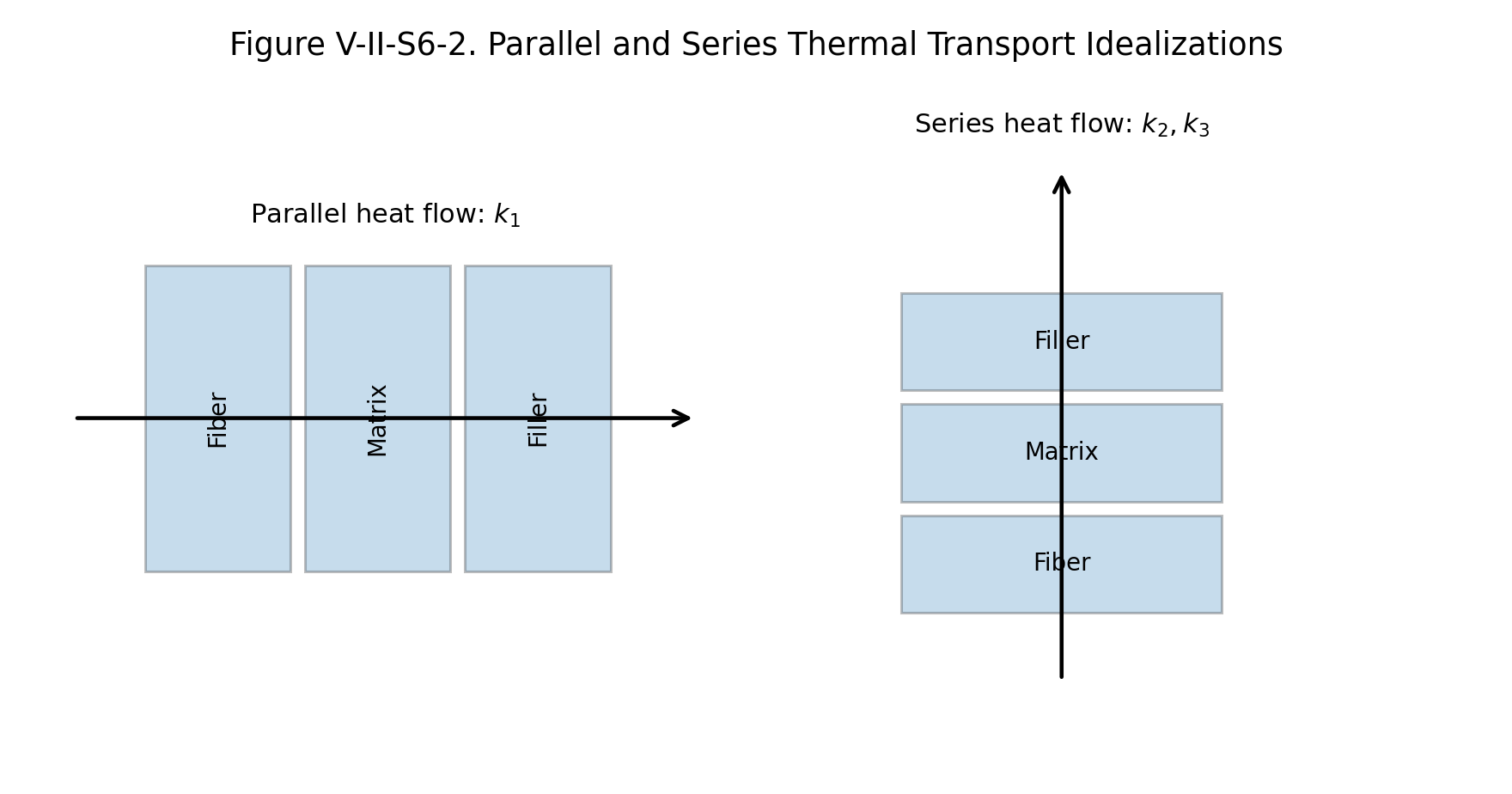
Figure V-II-S6-2. Parallel and series conductivity idealizations used as upper and lower engineering estimates.
6.4 Filler-Modified Matrix Conductivity
If filler is treated implicitly as a matrix modifier, the filled matrix conductivity is estimated using a Maxwell-type expression for dispersed particles,
Meaning, notation and theory source
Definitions and derivation: 6.4 Filler-Modified Matrix Conductivity
Meaning, notation and theory source
Definitions and derivation: 6.4 Filler-Modified Matrix Conductivity
Here is the effective conductivity of the filled resin, is the neat matrix conductivity, is the particulate filler conductivity, and is the filler volume fraction within the resin phase. This expression is consistent with the dilute spherical-inclusion limit and provides a stable engineering model for filled polymer matrices.
If filler is treated explicitly, the filler enters the multiphase conductivity equations through its own global volume fraction.
6.5 Mean-Field Conductivity Approximation
The thermal-conductivity analogue of a mean-field inclusion model can be expressed using a thermal concentration tensor ,
Meaning, notation and theory source
Definitions and derivation: 6.5 Mean-Field Conductivity Approximation
For an inclusion phase embedded in a matrix reference medium,
Meaning, notation and theory source
Definitions and derivation: 6.5 Mean-Field Conductivity Approximation
where is a thermal polarization tensor that depends on inclusion geometry and reference conductivity. The current Workbench-safe script does not perform a full tensor integration for ; instead, it uses robust engineering approximations based on the parallel, series, filled-matrix, and architecture-corrected expressions.
6.6 Self-Consistent Conductivity Statement
The full self-consistent conductivity problem would embed each phase in the unknown effective medium and solve
Meaning, notation and theory source
Definitions and derivation: 6.6 Self-Consistent Conductivity Statement
The corresponding fixed-point update is
Meaning, notation and theory source
Definitions and derivation: 6.6 Self-Consistent Conductivity Statement
6.7 Textile Architecture Effects
For woven fabrics, conductivity is redistributed by the warp and weft tow architecture. Let and denote the normalized warp and weft fractions. If denotes the tow-axis conductivity and denotes a transverse tow conductivity, the in-plane fabric conductivities are approximated as
Meaning, notation and theory source
Definitions and derivation: 6.7 Textile Architecture Effects
Meaning, notation and theory source
Definitions and derivation: 6.7 Textile Architecture Effects
where is the architecture-adjusted crimp factor. Through-thickness conductivity is reduced by the same architecture penalty in the implemented model,
Meaning, notation and theory source
Definitions and derivation: 6.7 Textile Architecture Effects
where is a small positive numerical floor. The same architecture framework supports plain weave, twill, satin, basket weave, leno weave, non-crimp stitched fabrics, and triaxial braids.
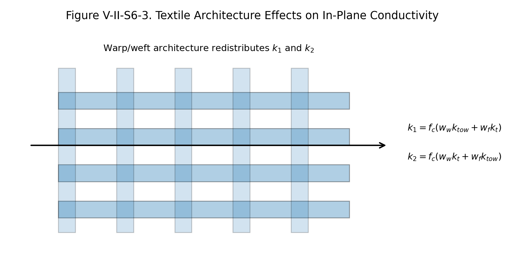
Figure V-II-S6-3. Textile architecture effects on in-plane thermal conductivity.
6.10 Verification Checks
The following checks are recommended for the thermal-conductivity implementation.
- If and no filler is present, the model must recover .
- If for aligned continuous fibers, must approach .
- If the void volume fraction increases, and must decrease.
- For a balanced fabric, and should approach each other.
- For an unbalanced fabric, should track the warp/weft weighting.
6.11 References
Chamis, C. C. (1983). Simplified composite micromechanics equations for hygral, thermal and mechanical properties. SAMPE Quarterly, 15, 14-23.
Mura, T. (1987). Micromechanics of Defects in Solids. Martinus Nijhoff.
Benveniste, Y. (1987). A new approach to the application of Mori-Tanaka’s theory in composite materials. Mechanics of Materials, 6, 147-157.
Dvorak, G. J. (2013). Micromechanics of Composite Materials. Springer.
Torquato, S. (2002). Random Heterogeneous Materials: Microstructure and Macroscopic Properties. Springer.
Jones, R. M. (1999). Mechanics of Composite Materials. Taylor & Francis.
3.4 CTE Micromechanics
Volume II - Section 7: Effective Thermal Expansion and Thermoelastic Micromechanics
7.1 Purpose and Scope
This section documents the coefficient of thermal expansion (CTE) models used by the Workbench micromechanics code. The thermal expansion module converts constituent thermal expansion data for fiber, matrix, filler, void, tow, and fabric phases into effective orthotropic engineering properties. The final outputs are the three material-axis thermal expansion coefficients (_1), (_2), and (_3), which are exported to both effective properties and Abaqus material cards.
The implementation is intentionally consistent with the mechanical micromechanics framework. The same volume fractions, fabric architecture flags, crimp factors, warp/weft weighting factors, and filler/void corrections used for stiffness prediction are also used to assemble thermoelastic material properties.
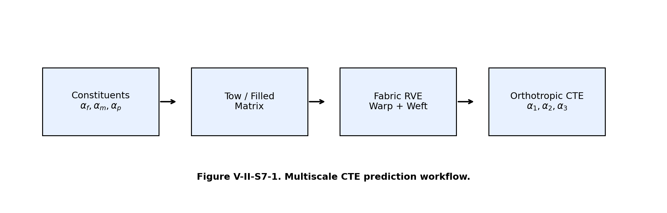
Figure V-II-S7-1. Multiscale CTE prediction workflow.
7.2 Thermal Strain and Thermoelastic Constitutive Law
For a homogeneous orthotropic material subjected to a temperature increment ΔT, the free thermal strain vector in engineering notation is written as
Meaning, notation and theory source
Definitions and derivation: 7.2 Thermal Strain and Thermoelastic Constitutive Law
where
Meaning, notation and theory source
Definitions and derivation: 7.2 Thermal Strain and Thermoelastic Constitutive Law
The thermoelastic stress-strain relation is
Meaning, notation and theory source
Definitions and derivation: 7.2 Thermal Strain and Thermoelastic Constitutive Law
where C is the effective stiffness matrix. This form is the basis
for the Abaqus *EXPANSION, TYPE=ORTHO export generated by
the solver script.
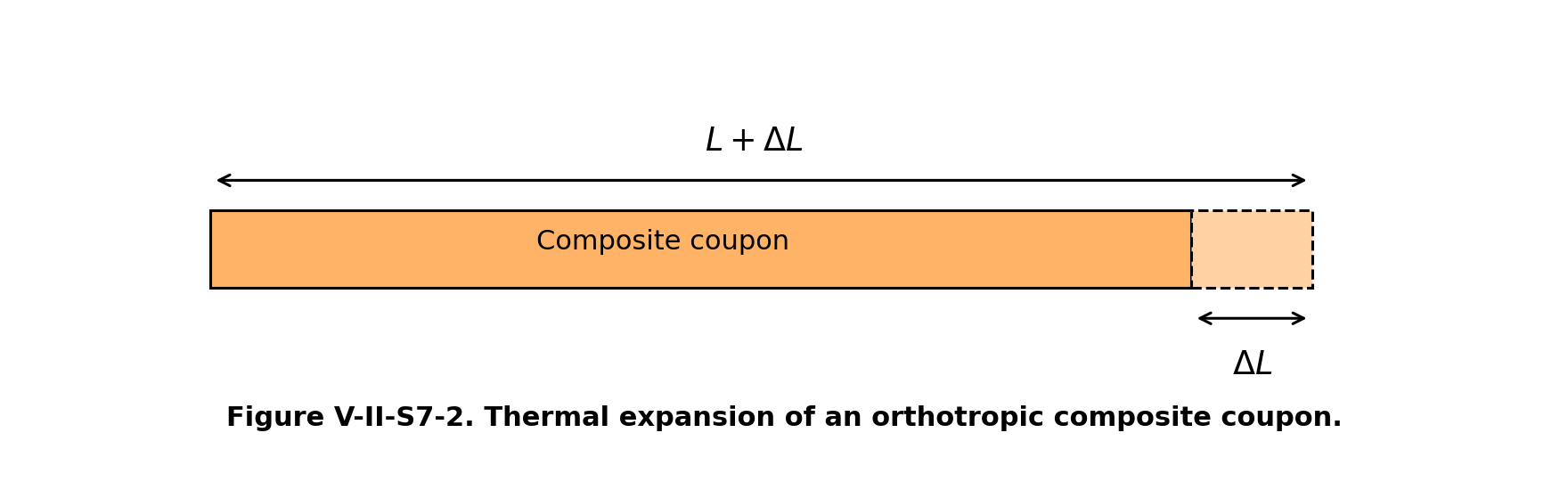
Figure V-II-S7-2. Thermal expansion of an orthotropic composite coupon.
7.3 Phase-Averaged Expansion in Composite Constituents
For a composite with fiber, matrix, filler, and void phases, the unconstrained volumetric expansion estimate is
Meaning, notation and theory source
Definitions and derivation: 7.3 Phase-Averaged Expansion in Composite Constituents
The phase-volume constraint is
Meaning, notation and theory source
Definitions and derivation: 7.3 Phase-Averaged Expansion in Composite Constituents
Because voids do not carry significant thermal stress, the model normally sets (_v=0) for the void contribution and accounts for voids primarily through dilution of load-carrying and heat-carrying phases.
7.4 Stiffness-Weighted Longitudinal CTE
For continuous fiber composites, axial expansion is constrained by the stiffness of the phases in the fiber direction. The longitudinal CTE estimate used by the model is therefore stiffness weighted:
Meaning, notation and theory source
Definitions and derivation: 7.4 Stiffness-Weighted Longitudinal CTE
This expression captures the fact that high-modulus fibers dominate axial expansion even when the matrix has a much larger unconstrained thermal expansion coefficient.
7.5 Transverse and Through-Thickness CTE Estimates
The current engineering implementation uses mixture-style transverse and through-thickness expansion estimates:
Meaning, notation and theory source
Definitions and derivation: 7.5 Transverse and Through-Thickness CTE Estimates
Meaning, notation and theory source
Definitions and derivation: 7.5 Transverse and Through-Thickness CTE Estimates
7.6 Filled-Matrix CTE
When the filler is treated implicitly as part of the resin-rich phase, the filled matrix CTE is estimated by phase averaging:
Meaning, notation and theory source
where (V_p^{res}) is the filler volume fraction inside the resin phase. This filled-matrix value is then used as the matrix phase input for subsequent fiber and fabric homogenization.
7.7 Fabric Architecture Effects on CTE
For textile composites, warp and weft directions exchange the roles of axial and transverse tow properties. The model uses architecture-weighted CTE assembly:
Meaning, notation and theory source
Definitions and derivation: 7.7 Fabric Architecture Effects on CTE
Meaning, notation and theory source
Definitions and derivation: 7.7 Fabric Architecture Effects on CTE
where (w_{warp}) and (w_{weft}) are normalized fabric architecture fractions satisfying
Meaning, notation and theory source
Definitions and derivation: 7.7 Fabric Architecture Effects on CTE
Crimp and architecture effects modify the mechanical constraints and thermal directions indirectly through the same factors used in stiffness assembly.
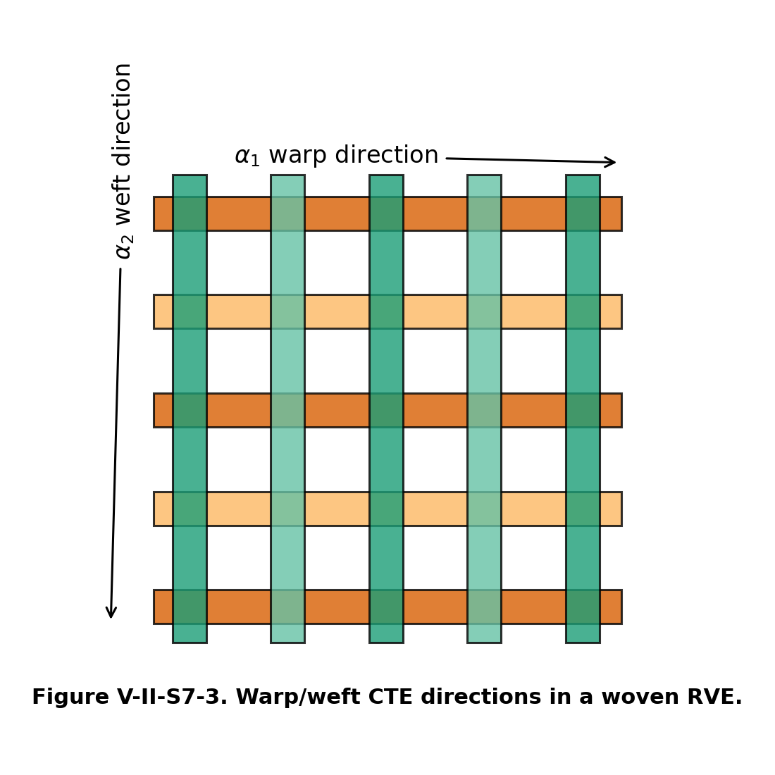
Figure V-II-S7-3. Warp/weft CTE directions in a woven RVE.
7.8 Architecture Library and CTE Interpretation
The fabric architecture flag controls the interpretation of the warp/weft CTE assembly. Plain weaves usually exhibit larger crimp and stronger interlacing effects. Satin weaves usually have lower interlacing and reduced tow waviness. Non-crimp fabrics preserve near-straight tow paths and therefore maintain stronger directional anisotropy. Triaxial braids introduce bias-angle effects that couple the two in-plane expansion directions.
The implemented fabric architecture set includes:
- plain weave,
- 2 by 2 twill,
- 4-harness satin,
- 5-harness satin,
- 8-harness satin,
- basket weave,
- leno weave,
- non-crimp biaxial stitched fabric,
- triaxial braid.
7.11 Representative CTE Trend
The stiffness-weighted expression causes the longitudinal CTE of carbon/epoxy composites to decrease rapidly with increasing fiber volume fraction because carbon fibers have low or negative axial CTE and high axial stiffness.
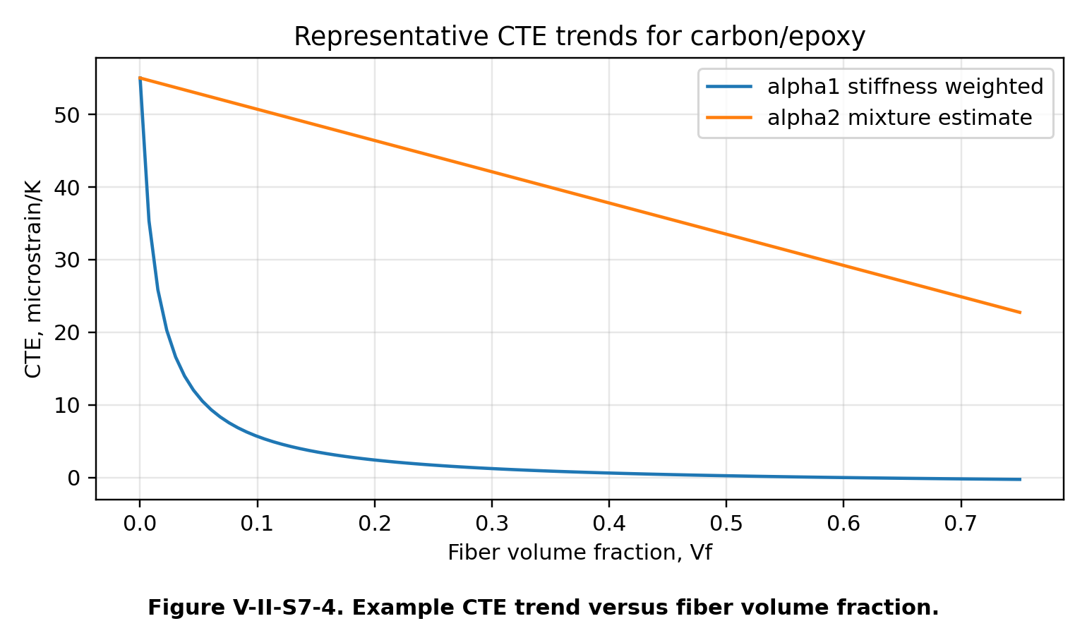
Figure V-II-S7-4. Example CTE trend versus fiber volume fraction.
7.12 Assumptions and Limitations
The current CTE implementation is an engineering micromechanics approximation. It is appropriate for rapid material-property prediction, Workbench integration, and finite-element preprocessing. It does not solve the full thermoelastic inclusion boundary-value problem for arbitrary ellipsoidal inclusions. For high-fidelity thermoelastic homogenization, the full fourth-order concentration tensors from Mori-Tanaka or self-consistent theory should be coupled directly to the phase eigenstrain tensors.
The implemented model assumes:
- small-strain linear thermoelasticity,
- temperature-independent constituent properties unless externally updated,
- orthotropic effective material axes,
- architecture correction factors shared with the mechanical model,
- voids contribute negligibly to stiffness and thermal expansion constraint.
7.13 References
- Jones, R. M. Mechanics of Composite Materials. Taylor & Francis, 1999.
- Chou, T. W. Microstructural Design of Fiber Composites. Cambridge University Press, 1992.
- Mura, T. Micromechanics of Defects in Solids. Martinus Nijhoff, 1987.
- Dvorak, G. J. Micromechanics of Composite Materials. Springer, 2013.
- Schapery, R. A. Thermal expansion coefficients of composite materials based on energy principles. Journal of Composite Materials, 1968.
- Rosen, B. W. Thermoelastic behavior of fiber composites. In Fiber Composite Materials, ASM, 1965.
- Hashin, Z. Analysis of composite materials - A survey. Journal of Applied Mechanics, 1983.
- Ishikawa, T. and Chou, T. W. Stiffness and strength behavior of woven fabric composites. Journal of Materials Science, 1982.
- Naik, N. K. Woven Fabric Composites. Technomic, 1994.
3.5 Semi-analytical aligned discontinuous-composite theory
Current Workbench models and compatibility
This theory library includes wider research formulations. Check the released model directory for selectable models, required inputs, limits and exercises. The event-driven RVE branch is not enabled in hosted Workbench.
Theories / Micromechanics / Aligned discontinuous fibers
Reference formulation — not enabled in hosted Workbench.This Revision 8 chapter documents a separate research formulation. Its event-driven breaks, nonlinear shear, RVE series coupling and stochastic failure are not selectable in hosted Workbench. Cox shear-lag elastic homogenization is available, not this failure model. Released models and connections ↗
1. Theory basis and role in CDS
Henry and Pimenta model aligned short-fiber material across specimen, RVE, fiber, neighboring-fiber interaction, and interaction-segment scales. Random fiber ends create nonuniform overlaps, matrix shear transfers load, fiber strength is stochastic, and final failure occurs when a local cluster becomes unstable.
The reference implementation associates this formulation with aligned-discontinuous material type 1 / criterion 6; this is not a selectable hosted Workbench path. Its specimen response supplies longitudinal ply stiffness and tensile strength to the common orthotropic ply property definition. Laminate ABD assembly and laminate-scale progressive degradation remain separate downstream operations.
2. Paper-to-CDS traceability
| Henry–Pimenta mechanism | Revision 8 status | CDS implementation |
|---|---|---|
| Random longitudinal fiber-end locations | Implemented | Each RVE draws one end location per fiber over the selected fiber length. |
| Square n × n aligned-fiber RVE | Implemented | The user controls fibers per row and the number of independent RVEs. |
| Four-nearest-neighbor topology | Implemented | Horizontal and vertical interactions are rebuilt from fiber ends and inserted breaks. |
| Generic nonlinear matrix constitutive law | Implemented | An optional piecewise-linear τ(γ) table is accepted; otherwise CDS builds an elastic-yield-friction law. |
| Broken and shear-lag interaction segments | Implemented | Same-fiber endpoints create broken segments; different-fiber endpoints create nonlinear shear-lag segments. |
| Length- and field-scaled Weibull strength | Implemented | Ordered thresholds use fiber/reference length, Weibull scale and shape, and stress-field correction. |
| Event-driven break insertion and rebuilding | Implemented | The governing break coordinate is inserted, its interaction is deactivated, and the network is rebuilt at the same strain. |
| Debonding and frictional pull-out toughness | Implemented | Resistance is integrated over realized overlaps from mode-II toughness and residual friction. |
| Dugdale critical-cluster instability | Implemented | Square clusters are screened with the nonlinear energy-release expression and physical cluster radius. |
| Specimen curve from RVEs in series | Implemented | RVE strains are interpolated at common stress and averaged; the first RVE cutoff governs. |
3. Interaction-segment mechanics
3.1 Discontinuity reconstruction
For each horizontal and vertical neighbor pair, CDS sorts both fiber ends and all inserted break coordinates. Consecutive discontinuities define the current interaction segments. If both endpoints belong to the same fiber, the segment is broken; if they belong to different fibers, load crosses the matrix through shear lag.
Equation detailsExplanation · variables · model connection · reference+
Relates interaction stress to strain in a segment bounded by discontinuities on the same fiber.
Model connectionSupplies the broken-segment response used in the length-weighted interaction strain.
Theory basisHenry and Pimenta (2017), reference formulation
3.2 Nonlinear shear lag
With fiber half-thickness T = φf/4 and effective matrix gap tm, the fiber stress difference follows:
Equation detailsExplanation · variables · model connection · reference+
Describes how the stress difference between neighboring fibers varies along an interaction segment. The active matrix-law branch determines the sign and stiffness used.
Model connectionProvides the nonlinear shear-lag segment response before segments are combined in series.
Theory basisHenry and Pimenta (2017), reference formulation
The active secant/tangent behavior comes from the selected piecewise-linear matrix law. The interaction stress is common to its segments, and their strain contributions are length-weighted in series. The weakest segment limits the interaction.
Equation detailsExplanation · variables · model connection · reference+
Averages segment strains by their lengths at a common interaction stress.
Model connectionConnects individual broken and shear-lag segments to the representative-volume response.
Theory basisHenry and Pimenta (2017), reference formulation
4. Progressive fiber-break events
Each fiber receives ordered Weibull thresholds. Length and stress-field scaling follow:
Equation detailsExplanation · variables · model connection · reference+
Expresses the probability of fiber failure with corrections for fiber length and the nonuniform stress field.
Model connectionGenerates the ordered fiber-strength thresholds that trigger break insertion and network rebuilding.
Theory basisHenry and Pimenta (2017), reference formulation
Four adjacent interactions generate the fiber peak. When that peak exceeds the current threshold, CDS inserts a break at the governing neighboring discontinuity at the end of the longest segment, advances the ordered threshold, deactivates the responsible interaction, and rebuilds the network without advancing applied strain. Events repeat until stable.
5. RVE, specimen, and cluster failure
Equation detailsExplanation · variables · model connection · reference+
Combines the horizontal and vertical interaction stresses with the matrix contribution to obtain the representative-volume stress.
Model connectionProduces each representative volume’s stress–strain curve for specimen assembly.
Theory basisHenry and Pimenta (2017), reference formulation
Independent RVEs are placed in series. At a common stress, their interpolated strains are averaged; the earliest RVE cutoff limits the specimen.
Equation detailsExplanation · variables · model connection · reference+
Averages representative-volume strains evaluated at the same axial stress.
Model connectionBuilds the specimen response from volumes in series; the earliest volume cutoff limits the specimen.
Theory basisHenry and Pimenta (2017), reference formulation
Cluster termination uses the nonlinear Dugdale energy release rate and the paper's cluster-radius scaling:
Equation detailsExplanation · variables · model connection · reference+
Evaluates nonlinear energy release for a damaged cluster and relates its physical radius to the fiber array.
Model connectionThe cluster energy release is compared with calibrated fracture resistance to determine instability.
Theory basisHenry and Pimenta (2017), reference formulation
Equation detailsExplanation · variables · model connection · reference+
Evaluates the debonding and frictional pull-out contributions for a realized overlap length.
Model connectionThese resistance contributions enter the critical-cluster instability assessment.
Theory basisHenry and Pimenta (2017), reference formulation
6. Connected workflow
- ConstituentsFiber elastic/Weibull data and matrix elastic, strength, toughness, friction, and optional τ(γ) data
- Stochastic geometryFiber length/diameter, volume fraction, n × n RVE, independent realizations, and seed
- Interaction networkEnds + breaks → broken/shear-lag segments → nonlinear segment series response
- Fiber eventsLocal peaks → ordered Weibull threshold → break insertion → network rebuild at the same strain
- RVE and specimenInteraction average → complete RVE curves → common-stress series coupling
- Cluster and ply property connectionDugdale cutoff → E1/Xt → 3D ply properties → laminate and structural analysis
7. What to supply and what to examine
| Study quantity | Physical meaning |
|---|---|
| Fiber variability and interactions | Specify fiber-strength statistics, representative-volume size, flaw assumptions and calibrated fracture resistance. |
| Matrix shear behavior | Supply measured shear strain and shear stress in Pa. Strain values must be nonnegative and strictly increasing. |
| Specimen response | Series-coupled specimen curves. |
| RVE response | RVE curves, break counts, active-interaction counts, and cutoff state. |
| Fiber-break events | Every progressive fiber-break event and governing interaction. |
| Critical clusters | Critical cluster location, size, JNL, and resistance. |
| Matrix shear law | Resolved matrix shear-law points and piecewise tangent. |
8. Calibration and validation boundary
- Calibrate the matrix shear law, Weibull scale/shape/reference length, stress-field correction, interface limit, mode-II toughness, and friction stress to the intended material state.
- RVE row count, RVE count, strain resolution, cluster limit, and flaw opportunities require convergence studies.
- Static and analytical release checks do not replace a complete model run or coupon validation.
- Use measured ply overrides when a qualified dataset should supersede a predicted property.
9. Primary reference
Henry, J., and Pimenta, S. (2017). “Semi-analytical simulation of aligned discontinuous composites.” Composites Science and Technology, 144, 230–244. https://doi.org/10.1016/j.compscitech.2017.01.027
3.6 Textile and Thermophysical Framework
Volume II – Textile and Thermophysical Micromechanics
Section 1 – Introduction and Multiscale Framework
1.1 Purpose and Scope
Volume II documents the textile, hybrid, and thermophysical extensions of the Workbench micromechanics solver model. Volume I established the elastic micromechanics foundation for continuous and discontinuous fiber composites. The present volume extends that foundation to woven, braided, stitched, and non-crimp fabric architectures, and to the effective thermophysical properties needed for coupled thermal and structural finite-element simulations.
The model treats the composite as a hierarchy of homogenization problems. Constituent fibers, polymer matrix, particulate filler, and void phases are first assembled into local material descriptions. These local descriptions are then homogenized into tow properties, textile representative volume element properties, and finally orthotropic lamina properties suitable for Abaqus material-card export.
The Volume II model branches predict the following quantities:
- effective orthotropic elastic constants influenced by fabric architecture;
- effective density;
- effective specific heat capacity;
- effective thermal conductivity in the material directions;
- effective coefficients of thermal expansion in the material directions;
- architecture factors for weave, braid, non-crimp, and stitched reinforcement systems;
- effective properties and Abaqus thermophysical material-card entries.
The goal is not to replace detailed finite-element textile unit-cell analysis. Instead, the intent is to provide a robust, deterministic, Workbench-safe engineering model that captures the dominant effects of tow homogenization, warp–weft balance, crimp, interlacing, fillers, voids, and orthotropic thermal response.
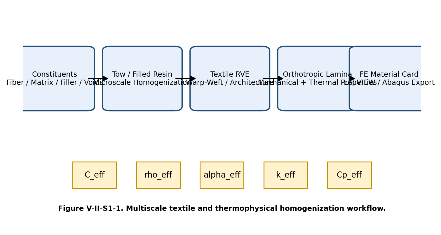
Figure V-II-S1-1. Multiscale textile and thermophysical homogenization workflow.
1.2 Multiscale Material Hierarchy
The model is organized around the assumption that each length scale may be represented by an effective property vector. The general homogenization mapping is written as
Meaning, notation and theory source
Definitions and derivation: 1.2 Multiscale Material Hierarchy
where is the property vector for phase , is its volume fraction, is the number of active phases, and denotes geometry or architecture descriptors such as weave type, crimp amplitude, warp/weft balance, stitch knockdown, binder fraction, or braid angle.
For the textile and thermophysical model, the phase-property vector is defined as
Meaning, notation and theory source
Definitions and derivation: 1.2 Multiscale Material Hierarchy
where is the stiffness tensor, is density, is the coefficient of thermal expansion tensor, is the thermal conductivity tensor, is specific heat capacity, and represents strength allowables when damage and failure calculations are enabled.
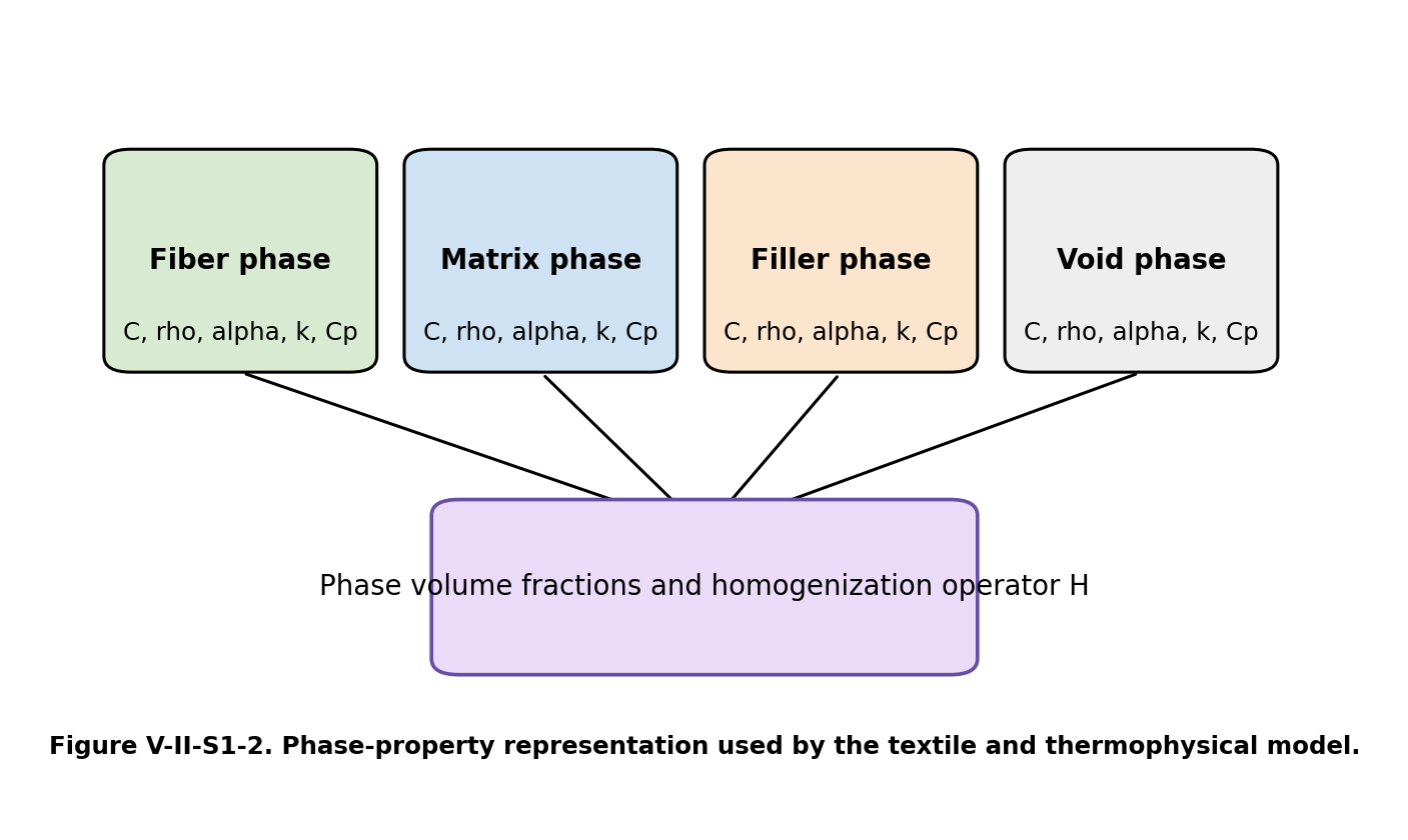
Figure V-II-S1-2. Phase-property representation used by the textile and thermophysical model.
1.3 Phase Volume Fractions
The phase fractions satisfy the conservation constraint
Meaning, notation and theory source
For the fiber–matrix–filler–void representation used in the solver implementation,
Meaning, notation and theory source
where is fiber volume fraction, is matrix volume fraction, is particulate filler volume fraction, and is void volume fraction.
When filler is treated as an implicit modifier of the resin phase, the model first constructs a filled-matrix property set and then performs fiber/tow/fabric homogenization using that modified matrix. When filler is treated explicitly, the filler remains a distinct phase in the phase list used for the homogenization calculation.
1.4 Textile Architecture as a Reduced-Order Descriptor
A detailed textile unit cell may require tow cross-section shape, nesting, local waviness, inter-tow resin pockets, contact surfaces, and through-thickness binder geometry. The implemented Workbench model reduces this complexity to a set of architecture descriptors that can be specified through scalar inputs:
Meaning, notation and theory source
Definitions and derivation: 1.4 Textile Architecture as a Reduced-Order Descriptor
where is the fabric architecture identifier, and are warp and weft weighting fractions, is a crimp factor, is an interlacing factor, is an in-plane shear factor, is a stitching knockdown factor, is binder or through-thickness reinforcement fraction, and is a bias or braid angle.
The architecture library in the current solver implementation includes plain weave, 2 by 2 twill, four-harness satin, five-harness satin, eight-harness satin, basket weave, leno weave, non-crimp biaxial stitched fabric, and triaxial braid. These options are implemented as engineering corrections rather than as a finite-element textile meshing scheme.
1.5 General Textile Homogenization Operator
The textile-level homogenization problem may be written in the compact form
Meaning, notation and theory source
Definitions and derivation: 1.5 General Textile Homogenization Operator
In the engineering implementation, this relationship is evaluated through warp–weft weighted tow properties modified by architecture factors. The same conceptual form is also used for conductivity and thermal expansion,
Meaning, notation and theory source
Definitions and derivation: 1.5 General Textile Homogenization Operator
and
Meaning, notation and theory source
Definitions and derivation: 1.5 General Textile Homogenization Operator
This unified notation is useful because all material properties ultimately feed the same finite-element material description.
1.7 Volume II Output Philosophy
The final orthotropic property vector assembled by the Volume II branches is
Meaning, notation and theory source
The effective thermophysical properties are exported to Abaqus using the material-card blocks
Meaning, notation and theory source
1.8 Assumptions and Limitations
The Volume II formulation is a reduced-order engineering homogenization model. The principal assumptions are:
- tow properties can be represented by homogenized orthotropic engineering constants;
- textile architecture can be represented using warp/weft weights and architecture correction factors;
- crimp and interlacing are treated as stiffness and shear knockdown factors rather than explicit curved tow finite elements;
- filler and void phases are represented through effective phase-volume terms;
- thermophysical properties are homogenized through volume averaging, series/parallel conductivity estimates, and architecture corrections;
- all outputs are deterministic scalar, vector, matrix, or string quantities suitable for Workbench and Abaqus export.
These assumptions make the method much faster than detailed textile finite-element unit-cell analysis, but they also limit its ability to capture local tow contact, resin pocket stress concentration, inter-tow delamination, nesting effects, local permeability, and nonlinear compaction.
1.9 Section Summary
Section 1 defines the multiscale and software framework for Volume II. The following sections document the individual textile and thermophysical model components: textile representative volume elements, fabric architecture factors, warp–weft averaging, crimp correction, filled matrix micromechanics, void effects, density, specific heat, thermal conductivity, thermal expansion, and final orthotropic property assembly.
References
Advani, S. G., and Tucker, C. L. III (1987). The use of tensors to describe and predict fiber orientation in short fiber composites. Journal of Rheology, 31, 751–784.
Chou, T.-W. (1992). Microstructural Design of Fiber Composites. Cambridge University Press.
Dvorak, G. J. (2013). Micromechanics of Composite Materials. Springer.
Ishikawa, T., and Chou, T.-W. (1982). Stiffness and strength behavior of woven fabric composites. Journal of Materials Science, 17, 3211–3220.
Jones, R. M. (1999). Mechanics of Composite Materials, 2nd ed. Taylor & Francis.
Mura, T. (1987). Micromechanics of Defects in Solids, 2nd ed. Martinus Nijhoff.
Naik, N. K. (1994). Woven Fabric Composites. Technomic.
Whitcomb, J. D. (2001). Three-dimensional stress analysis of plain weave composites. Composite Materials: Fatigue and Fracture, ASTM STP.
3.7 Fabric Micromechanics Theory
2. Fabric Micromechanics Theory
2.1 Scope and purpose
This section documents the fabric micromechanics branch of the Workbench solver composite-material model. The fabric branch extends the elastic micromechanics framework of Volume I from unidirectional and discontinuous reinforcement to textile architectures. The current implementation supports common woven, stitched, non-crimp, and braided fabrics using a reduced-order representative-volume-element (RVE) framework. The goal is not to resolve every tow cross-section with a mesoscopic finite-element mesh. Instead, the model provides a fast engineering homogenization suitable for material screening, Workbench embedding, and automatic finite-element material-card generation.
For a woven or textile composite, choose the fabric family that represents the reinforcement. Architecture-specific factors then modify tow-dominated stiffness, in-plane shear response, thermophysical properties, and through-thickness reinforcement contributions. This section describes the theory behind those factors and explains how the model maps textile architecture into final orthotropic engineering constants.
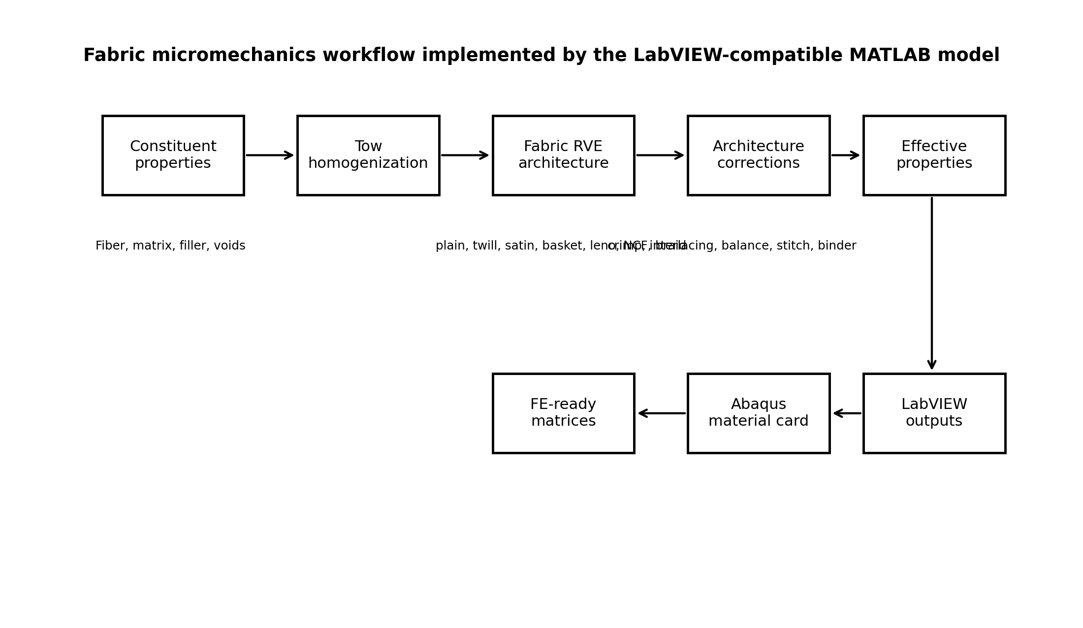
Figure V-II-S2-1. Fabric micromechanics workflow implemented in the Workbench solver model.
2.2 Textile composite scale hierarchy
The fabric formulation assumes three nested scales. At the constituent scale, fiber, matrix, filler, and void properties are specified independently. At the tow scale, fibers and matrix are homogenized into an equivalent orthotropic tow. At the textile scale, warp, weft, bias, stitch, and binder contributions are assembled into an effective fabric lamina.
The homogenization chain is represented as
Meaning, notation and theory source
Definitions and derivation: 2.2 Textile composite scale hierarchy
where , , and are the fiber, matrix, and particle property sets, respectively; , , , and are fiber, matrix, particle, and void volume fractions; is the selected tow homogenization model; and is the textile-level homogenization operator.
The final fabric property vector is
Meaning, notation and theory source
Definitions and derivation: 2.2 Textile composite scale hierarchy
2.3 Representative volume element definition
A textile RVE is the smallest repeating domain that preserves the relevant fabric architecture. The RVE contains a warp tow family, a weft tow family, matrix-rich pockets, and optional binder or stitching reinforcement. For non-crimp fabrics and triaxial braids, the RVE additionally contains bias tow families.
The phase volume-fraction constraint is
Meaning, notation and theory source
Definitions and derivation: 2.3 Representative volume element definition
At the fabric level, the tow fractions satisfy
Meaning, notation and theory source
Definitions and derivation: 2.3 Representative volume element definition
For a two-family woven fabric without explicit bias or binder phases,
Meaning, notation and theory source
Definitions and derivation: 2.3 Representative volume element definition
Balanced woven fabrics use
Meaning, notation and theory source
Definitions and derivation: 2.3 Representative volume element definition
whereas unbalanced fabrics use architecture- or user-specified
values. In the solver implementation, this weighting is controlled by
fabric_warp_bias_fraction,
woven_warp_volume_fraction, and
woven_weft_volume_fraction.
2.4 Supported fabric architecture library
The following fabric architectures are supported.
| Architecture | Primary modeling effect |
|---|---|
| User-defined textile | User-defined correction factors |
| Plain weave | High interlacing, high crimp, stable balanced response |
| 2×2 twill | Moderate interlacing, moderate crimp, improved drape |
| 4-harness satin | Low interlacing, lower crimp |
| 5-harness satin | Lower interlacing than 4HS |
| 8-harness satin | Low interlacing, high tow straightness |
| Basket weave | Grouped tows, reduced interlacing density |
| Leno weave | Locked yarns, high geometric stability, stronger yarn distortion |
| Non-crimp biaxial stitched fabric | Low tow crimp, stitch knockdown included |
| Triaxial braid | Axial and bias tow families with angle-dependent contribution |
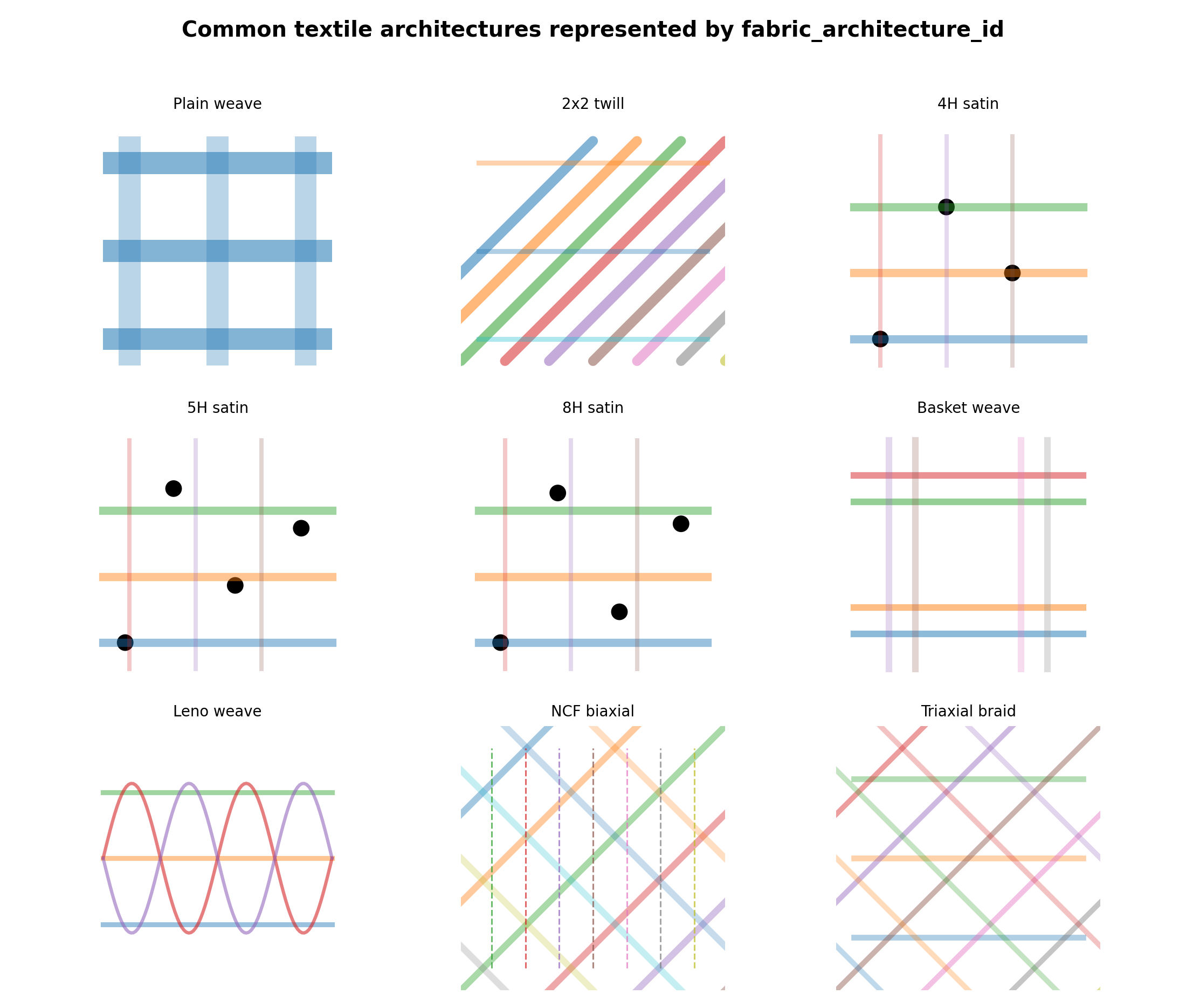
Figure V-II-S2-2. Common textile architectures represented in the fabric branch.
2.5 Tow homogenization
The tow is treated as a unidirectional composite sub-material. The selected constituent-level micromechanics model produces tow properties from the fiber and matrix properties. In high-level operator form,
Meaning, notation and theory source
where is the fiber volume fraction inside the tow.
The axial tow modulus used in the implemented engineering approximation is
Meaning, notation and theory source
A transverse tow modulus may be estimated using a Halpin-Tsai-like expression,
Meaning, notation and theory source
with
Meaning, notation and theory source
The same tow-level concept is applied to shear properties,
Meaning, notation and theory source
These tow-level properties become the input to the fabric-level homogenization step.
2.6 Warp-weft stiffness assembly
The fabric stiffness is assembled from warp and weft tow contributions. For a balanced woven architecture, the warp and weft fractions are equal. For an unbalanced fabric, the weighting is user-defined or architecture-derived.
The normalized tow-family fractions are
Meaning, notation and theory source
Definitions and derivation: 2.6 Warp-weft stiffness assembly
The implemented in-plane Young’s moduli are represented by
Meaning, notation and theory source
Definitions and derivation: 2.6 Warp-weft stiffness assembly
Meaning, notation and theory source
Definitions and derivation: 2.6 Warp-weft stiffness assembly
where is the architecture-adjusted crimp factor and is the balance factor. The through-thickness modulus is treated as a tow-transverse-dominated quantity modified by interlacing and optional binder reinforcement,
Meaning, notation and theory source
Definitions and derivation: 2.6 Warp-weft stiffness assembly
where is the interlacing penalty factor.
2.7 Crimp, interlacing, balance, and shear correction factors
Fabric architecture influences stiffness through geometric tow waviness and the number of over-under interlacings. The model uses reduced-order scalar correction factors rather than explicit meso-scale finite-element tow geometry.
The crimp factor is modeled as a decreasing function of the tow waviness amplitude ratio,
Meaning, notation and theory source
Definitions and derivation: 2.7 Crimp, interlacing, balance, and shear correction factors
where is tow waviness amplitude, is crimp wavelength, and is an architecture-dependent constant. Plain weaves use a larger effective because they interlace more frequently, while satin weaves use smaller values because they have longer floats and lower interlacing density.
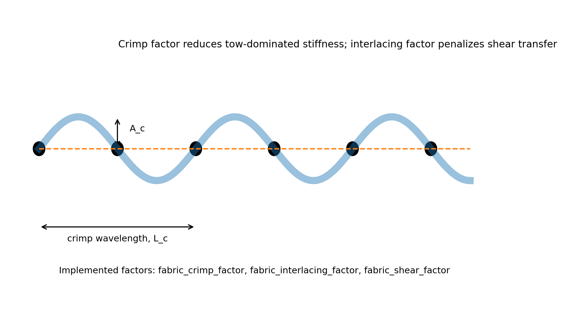
Figure V-II-S2-3. Crimp and interlacing correction concept used by the fabric branch.
The balance factor is defined from warp and weft fractions,
Meaning, notation and theory source
Definitions and derivation: 2.7 Crimp, interlacing, balance, and shear correction factors
This factor approaches unity for balanced fabrics and decreases as the architecture becomes strongly warp- or weft-dominated.
The interlacing penalty is represented by
Meaning, notation and theory source
Definitions and derivation: 2.7 Crimp, interlacing, balance, and shear correction factors
where is the architecture interlacing factor and is a calibration constant. The in-plane shear correction is expressed as
Meaning, notation and theory source
Definitions and derivation: 2.7 Crimp, interlacing, balance, and shear correction factors
where is the architecture shear factor and is the averaged tow-level shear modulus.
2.8 Architecture-specific interpretation
Plain weave has the highest interlacing density among the common balanced fabrics. It therefore receives the largest crimp and interlacing penalties. Twill fabrics reduce the interlacing frequency and improve drape, so the stiffness knockdown is less severe. Satin fabrics introduce longer tow floats, which reduce crimp and preserve tow axial stiffness but may reduce fabric stability during handling. Basket weaves group tows and reduce crossing density; leno weaves lock yarns together and improve dimensional stability but increase local yarn distortion. Non-crimp fabrics preserve tow straightness and therefore use very low crimp penalties, but stitching effects are included through a stitch knockdown factor. Triaxial braids include a bias-angle contribution that redistributes stiffness and increases in-plane shear coupling.
The architecture-dependent stiffness correction can be summarized as
Meaning, notation and theory source
Definitions and derivation: 2.8 Architecture-specific interpretation
where denotes the reduced-order architecture operator.
2.9 Non-crimp fabrics and triaxial braids
For non-crimp stitched fabrics, the tow path remains comparatively straight, and the crimp correction is weak. The stiffness is primarily reduced by the stitching knockdown factor,
Meaning, notation and theory source
Definitions and derivation: 2.9 Non-crimp fabrics and triaxial braids
For triaxial braids, a bias angle introduces additional axial-to-shear coupling. The implemented high-level bias contribution is represented by
Meaning, notation and theory source
Definitions and derivation: 2.9 Non-crimp fabrics and triaxial braids
The in-plane shear modulus is then increased by a bias contribution,
Meaning, notation and theory source
Definitions and derivation: 2.9 Non-crimp fabrics and triaxial braids
where is an engineering calibration coefficient.
2.10 Through-thickness binder and stitching effects
Through-thickness binder yarns or stitches can contribute to , , and . The model represents this contribution by a scalar binder volume fraction :
Meaning, notation and theory source
Definitions and derivation: 2.10 Through-thickness binder and stitching effects
Meaning, notation and theory source
Definitions and derivation: 2.10 Through-thickness binder and stitching effects
Meaning, notation and theory source
Definitions and derivation: 2.10 Through-thickness binder and stitching effects
In the current solver model, the binder stiffness is approximated
using the fiber axial and shear properties, and
is supplied by fabric_z_binder_volume_fraction.
2.11 Thermophysical extension for fabric architectures
The same architecture concept is applied to thermal conductivity and coefficient of thermal expansion. The warp- and weft-weighted conductivity components are
Meaning, notation and theory source
Definitions and derivation: 2.11 Thermophysical extension for fabric architectures
Meaning, notation and theory source
Definitions and derivation: 2.11 Thermophysical extension for fabric architectures
and
Meaning, notation and theory source
Definitions and derivation: 2.11 Thermophysical extension for fabric architectures
The in-plane coefficients of thermal expansion are assembled as
Meaning, notation and theory source
Definitions and derivation: 2.11 Thermophysical extension for fabric architectures
Meaning, notation and theory source
Definitions and derivation: 2.11 Thermophysical extension for fabric architectures
The scalar density and specific heat are not strongly dependent on fabric interlacing and are instead determined by phase volume fractions as described in Section 5 of this volume.
2.13 Assumptions and limitations
The fabric model is an engineering homogenization model. It does not solve local meso-scale tow contact, resin-pocket stress concentrations, yarn compaction, cure-dependent tow nesting, or finite-strain shear locking. The architecture factors provide a compact way to represent first-order fabric effects within a Workbench-safe micromechanics script. Detailed textile unit-cell finite-element analysis may be required for local damage initiation, matrix pocket cracking, tow debonding, and compaction modeling.
Despite these limitations, the model is appropriate for rapid architecture screening, laminate-level finite-element material definition, preliminary material design, and parametric comparison of common fabric types.
2.14 References
- Ishikawa, T., and Chou, T.-W. Stiffness and strength behavior of woven fabric composites. Journal of Materials Science, 1982.
- Ishikawa, T., and Chou, T.-W. One-dimensional micromechanical analysis of woven fabric composites. AIAA Journal, 1983.
- Chou, T.-W. Microstructural Design of Fiber Composites. Cambridge University Press, 1992.
- Naik, N. K. Woven Fabric Composites. Technomic Publishing, 1994.
- Whitcomb, J. D. Three-dimensional stress analysis of plain weave composites. Composite Materials: Testing and Design, ASTM STP series.
- Cox, B. N., and Flanagan, G. Handbook of Analytical Methods for Textile Composites. NASA Contractor Report, 1997.
- Lomov, S. V., Ivanov, D. S., Verpoest, I., et al. Meso-FE modelling of textile composites: Road map, data flow and algorithms. Composites Science and Technology, 2007.
- Advani, S. G., and Tucker, C. L. III. The use of tensors to describe and predict fiber orientation in short fiber composites. Journal of Rheology, 1987.
- Jones, R. M. Mechanics of Composite Materials. Taylor & Francis, 1999.
- Daniel, I. M., and Ishai, O. Engineering Mechanics of Composite Materials. Oxford University Press, 2006.
3.8 Warp-Weft Averaging and Crimp Correction
Volume II - Section 3
Warp-Weft Averaging and Crimp Correction in Fabric Micromechanics
3.1 Purpose and Scope
This section documents the fabric-level homogenization step used in the Workbench solver micromechanics model. Volume I defines the constituent and tow-level elastic micromechanics. Volume II Section 2 defines the textile architecture library. The present section describes how the homogenized tow properties are combined into effective fabric properties using warp-weft weighting, crimp correction, interlacing correction, shear correction, and optional through-thickness binder contributions.
This model applies to woven or textile composites. Select the fabric architecture that represents the reinforcement.
The fabric architecture options are listed in Table 3.1.
| Fabric architecture | Primary correction features |
|---|---|
| User-defined | User-specified crimp/interlacing factors |
| Plain weave | High interlacing, high crimp |
| 2 x 2 twill | Moderate interlacing, moderate crimp |
| 4-harness satin | Low interlacing, low crimp |
| 5-harness satin | Lower interlacing, lower crimp |
| 8-harness satin | Very low interlacing, very low crimp |
| Basket weave | Grouped-tow behavior, moderate locking |
| Leno weave | High yarn locking and distortion |
| Non-crimp biaxial stitched fabric | Low crimp with stitch knockdown |
| Triaxial braid | Bias reinforcement contribution |
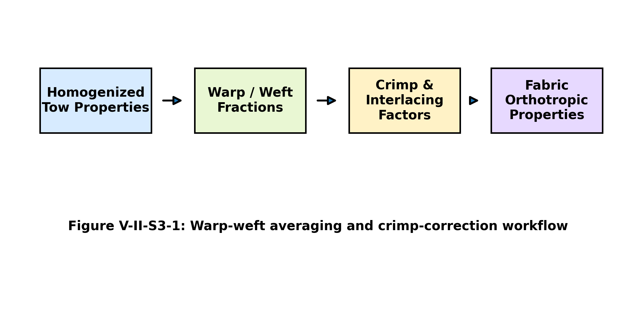
Figure V-II-S3-1. Warp-weft averaging and crimp-correction workflow.
3.2 Tow Properties Passed from Constituent Micromechanics
Each fabric architecture begins with an equivalent homogenized tow. The tow may be obtained from any micromechanics branch described in Volume I, including rule of mixtures, Halpin-Tsai, Mori-Tanaka approximation, or the self-consistent engineering approximation. The homogenized tow property vector is represented by
Meaning, notation and theory source
Definitions and derivation: 3.2 Tow Properties Passed from Constituent Micromechanics
The tow homogenization operator can be written abstractly as
Meaning, notation and theory source
Definitions and derivation: 3.2 Tow Properties Passed from Constituent Micromechanics
where ({f}) and ({m}) are the fiber and matrix property
vectors and (V_{f}^{}) is the tow fiber volume fraction. In the solver
implementation, this input is represented by
woven_tow_fiber_volume_fraction.
The simplified tow axial modulus used in the woven branch is
Meaning, notation and theory source
Definitions and derivation: 3.2 Tow Properties Passed from Constituent Micromechanics
where (E_m^*) is the matrix or filled-matrix modulus. The transverse tow modulus is represented using the same Halpin-type interaction form used elsewhere in the model,
Meaning, notation and theory source
Definitions and derivation: 3.2 Tow Properties Passed from Constituent Micromechanics
with
Meaning, notation and theory source
Definitions and derivation: 3.2 Tow Properties Passed from Constituent Micromechanics
These expressions are engineering approximations used to keep the Workbench implementation robust. They are consistent with the classical tow-property hierarchy used in textile composite micromechanics.
3.3 Warp and Weft Coordinate Systems
The fabric is modeled as two interacting orthotropic tow families. Warp tows are aligned nominally with the material 1-direction, while weft tows are aligned nominally with the material 2-direction. The effective fabric response is assembled from the contributions of both families.
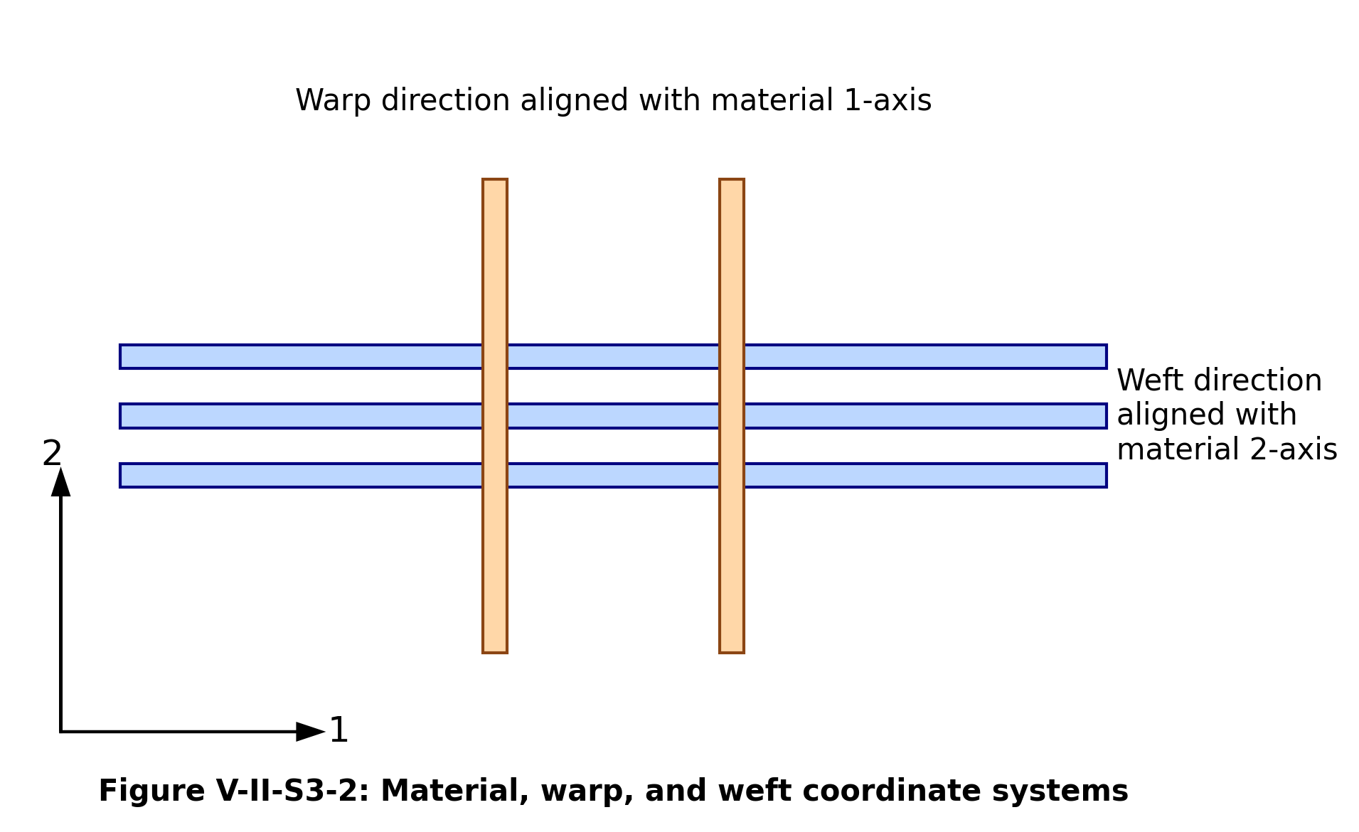
Figure V-II-S3-2. Material, warp, and weft coordinate systems.
The normalized warp and weft weights are
Meaning, notation and theory source
Definitions and derivation: 3.3 Warp and Weft Coordinate Systems
Meaning, notation and theory source
Definitions and derivation: 3.3 Warp and Weft Coordinate Systems
with
Meaning, notation and theory source
Definitions and derivation: 3.3 Warp and Weft Coordinate Systems
In the code these quantities are initialized using
woven_warp_volume_fraction and
woven_weft_volume_fraction, then optionally overwritten by
fabric_warp_bias_fraction. A balanced fabric has
Meaning, notation and theory source
Definitions and derivation: 3.3 Warp and Weft Coordinate Systems
An unbalanced fabric is represented by
Meaning, notation and theory source
Definitions and derivation: 3.3 Warp and Weft Coordinate Systems
3.4 Warp-Weft Stiffness Averaging
The effective axial moduli are computed by assigning the tow axial stiffness to the direction in which a tow family runs and assigning the transverse tow stiffness to the orthogonal direction. The high-level uncorrected averaging model is
Meaning, notation and theory source
Definitions and derivation: 3.4 Warp-Weft Stiffness Averaging
Meaning, notation and theory source
Definitions and derivation: 3.4 Warp-Weft Stiffness Averaging
Meaning, notation and theory source
Definitions and derivation: 3.4 Warp-Weft Stiffness Averaging
This captures the first-order architecture effect: increasing the warp fraction increases (E_1), while increasing the weft fraction increases (E_2). For balanced fabrics, the in-plane moduli become nearly equal if the warp and weft tow properties are equivalent.
The in-plane shear modulus is represented by
Meaning, notation and theory source
Definitions and derivation: 3.4 Warp-Weft Stiffness Averaging
where (G_{12}^{}) is the selected matrix/tow interaction shear estimate from the micromechanics branch. The through-thickness shear moduli are represented by the corresponding matrix-constrained terms,
Meaning, notation and theory source
Definitions and derivation: 3.4 Warp-Weft Stiffness Averaging
3.5 Tow Crimp Geometry
Tow crimp describes the waviness of a tow centerline relative to a straight reference direction. A sinusoidal representation provides a compact engineering measure of waviness,
Meaning, notation and theory source
where (A) is crimp amplitude and (L_c) is crimp wavelength.
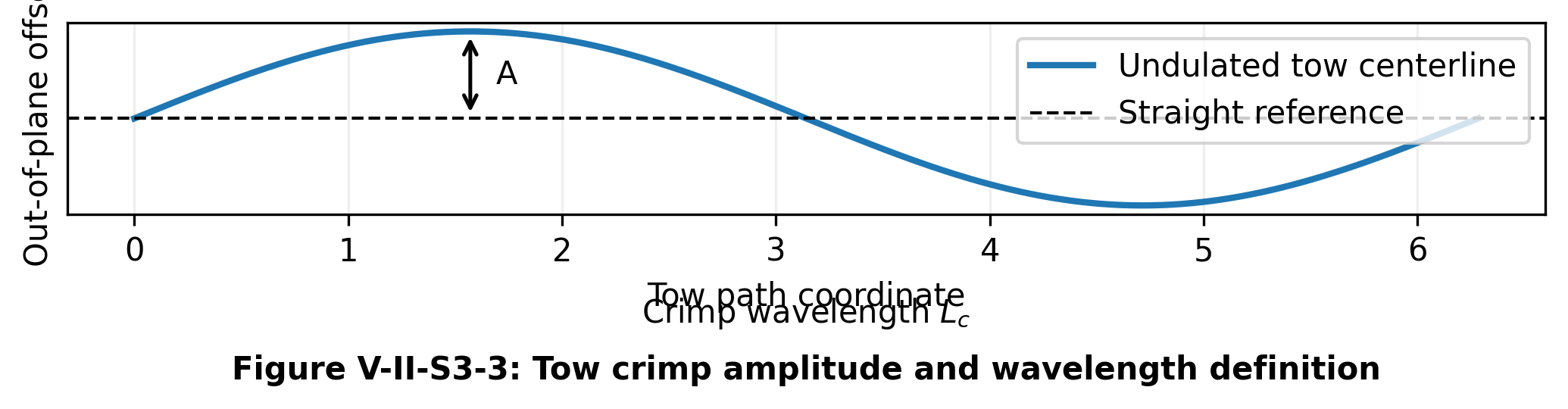
Figure V-II-S3-3. Tow crimp amplitude and wavelength definition.
The nondimensional crimp amplitude ratio used by the model is
Meaning, notation and theory source
A crimp knockdown factor is then introduced as
Meaning, notation and theory source
where (_c) is an architecture-dependent coefficient. This expression has the correct limiting behavior:
Meaning, notation and theory source
and
Meaning, notation and theory source
The code uses architecture-specific values of (_c). Plain weave and leno weave use stronger crimp penalties. Satin and non-crimp architectures use smaller penalties because the tows are straighter.
3.6 Architecture-Specific Correction Factors
The solver model applies four primary architecture correction factors:
Meaning, notation and theory source
Definitions and derivation: 3.6 Architecture-Specific Correction Factors
Meaning, notation and theory source
Definitions and derivation: 3.6 Architecture-Specific Correction Factors
Meaning, notation and theory source
Definitions and derivation: 3.6 Architecture-Specific Correction Factors
Meaning, notation and theory source
Definitions and derivation: 3.6 Architecture-Specific Correction Factors
The balance factor is computed from the warp/weft fraction difference,
Meaning, notation and theory source
Definitions and derivation: 3.6 Architecture-Specific Correction Factors
The architecture factors provide an engineering reduction of the textile unit-cell mechanics into scalar modifiers. The corrected in-plane moduli are
Meaning, notation and theory source
Definitions and derivation: 3.6 Architecture-Specific Correction Factors
Meaning, notation and theory source
Definitions and derivation: 3.6 Architecture-Specific Correction Factors
and the through-thickness modulus is
Meaning, notation and theory source
Definitions and derivation: 3.6 Architecture-Specific Correction Factors
where the interlacing penalty used in the code is
Meaning, notation and theory source
Definitions and derivation: 3.6 Architecture-Specific Correction Factors
The corrected shear moduli are
Meaning, notation and theory source
Definitions and derivation: 3.6 Architecture-Specific Correction Factors
Meaning, notation and theory source
Definitions and derivation: 3.6 Architecture-Specific Correction Factors
Meaning, notation and theory source
Definitions and derivation: 3.6 Architecture-Specific Correction Factors
Figure V-II-S3-4 summarizes representative relative values used for common fabric families.
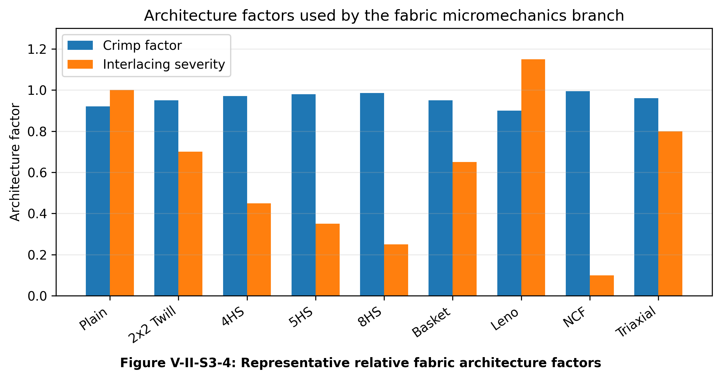
Figure V-II-S3-4. Representative relative fabric architecture factors.
3.7 Common Architecture Behavior
The architecture factors are selected to reproduce expected trends among common textile composites:
- Plain weave has high interlacing, higher tow crimp, and lower in-plane shear mobility.
- Twill weave has lower interlacing than plain weave and therefore a smaller crimp penalty.
- Satin weaves reduce interlacing further, increasing axial tow efficiency.
- Basket weave behaves like a grouped-tow plain weave with reduced interlacing density.
- Leno weave has strong tow locking and higher local yarn distortion.
- Non-crimp stitched fabric has low crimp but includes a stitch knockdown factor.
- Triaxial braid includes a bias-fiber contribution that increases in-plane coupling and shear response.
For triaxial braid architectures, the bias contribution is represented by
Meaning, notation and theory source
Definitions and derivation: 3.7 Common Architecture Behavior
where (_b) is the braid bias angle. The in-plane shear modulus is then increased according to
Meaning, notation and theory source
Definitions and derivation: 3.7 Common Architecture Behavior
For non-crimp fabric architectures, the stitch knockdown factor (f_{}) modifies the tow-dominated response,
Meaning, notation and theory source
Definitions and derivation: 3.7 Common Architecture Behavior
3.8 Through-Thickness Binder and Stitch Contribution
An optional through-thickness binder or stitch volume fraction can be used to increase through-thickness stiffness and shear stiffness. If (V_b) is the binder volume fraction, then
Meaning, notation and theory source
Definitions and derivation: 3.8 Through-Thickness Binder and Stitch Contribution
Meaning, notation and theory source
Definitions and derivation: 3.8 Through-Thickness Binder and Stitch Contribution
Meaning, notation and theory source
Definitions and derivation: 3.8 Through-Thickness Binder and Stitch Contribution
This is not a full three-dimensional woven unit-cell model, but it provides a useful engineering correction for stitched, 3D woven, and binder-stabilized textile preforms.
3.9 Thermophysical Warp-Weft Averaging
Thermal conductivity is treated using the same architecture logic. Before fabric correction, the longitudinal and transverse conductivity estimates are
Meaning, notation and theory source
Definitions and derivation: 3.9 Thermophysical Warp-Weft Averaging
Meaning, notation and theory source
Definitions and derivation: 3.9 Thermophysical Warp-Weft Averaging
The corrected in-plane conductivities are
Meaning, notation and theory source
Definitions and derivation: 3.9 Thermophysical Warp-Weft Averaging
Meaning, notation and theory source
Definitions and derivation: 3.9 Thermophysical Warp-Weft Averaging
with the through-thickness value reduced by the crimp-dominated transverse transfer factor,
Meaning, notation and theory source
Definitions and derivation: 3.9 Thermophysical Warp-Weft Averaging
The coefficients of thermal expansion are averaged as
Meaning, notation and theory source
Definitions and derivation: 3.9 Thermophysical Warp-Weft Averaging
Meaning, notation and theory source
Definitions and derivation: 3.9 Thermophysical Warp-Weft Averaging
3.11 Recommended Use
The fabric model is intended for engineering material-property generation, early design, sensitivity studies, and Workbench-driven material screening. It is appropriate when the user needs fast predictions across fabric families without constructing detailed textile finite-element RVEs. For final allowables, the model should be calibrated to coupon data and validated against the specific textile architecture, resin system, compaction state, and cure process.
References
- Ishikawa, T., and Chou, T.-W. “Stiffness and strength behaviour of woven fabric composites.” Journal of Materials Science, 1982.
- Ishikawa, T., and Chou, T.-W. “One-dimensional micromechanical analysis of woven fabric composites.” AIAA Journal, 1983.
- Chou, T.-W. Microstructural Design of Fiber Composites. Cambridge University Press, 1992.
- Naik, N. K. Woven Fabric Composites. Technomic, 1994.
- Whitcomb, J. D. “Three-dimensional stress analysis of plain weave composites.” Composite Materials: Testing and Design, ASTM STP, 1990s.
- Bogdanovich, A. E., and Pastore, C. M. Mechanics of Textile and Laminated Composites. Chapman & Hall, 1996.
- Advani, S. G., and Tucker, C. L. “The use of tensors to describe and predict fiber orientation in short fiber composites.” Journal of Rheology, 1987.
- Cox, H. L. “The elasticity and strength of paper and other fibrous materials.” British Journal of Applied Physics, 1952.
- Jones, R. M. Mechanics of Composite Materials. Taylor & Francis, 1999.
- Daniel, I. M., and Ishai, O. Engineering Mechanics of Composite Materials. Oxford University Press, 2006.
3.9 Filled Matrix, Hybrid, and Void Micromechanics
Volume II – Section 4
Filled-Matrix, Hybrid Reinforcement, and Void Micromechanics
4.1 Purpose and Scope
The section covers four related capabilities:
- implicit filler modification of the polymer matrix;
- explicit treatment of filler as a separate phase;
- hybrid fiber or hybrid tow property assembly; and
- void effects on stiffness, density, conductivity, and heat capacity.
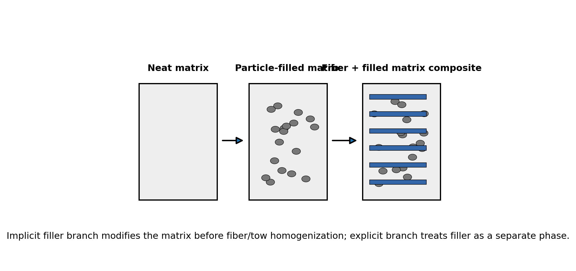
Figure V-II-S4-1. Filled-matrix homogenization workflow. The implicit branch modifies the resin before tow or fabric homogenization; the explicit branch retains filler as an independent phase.
4.2 Phase Definitions and Volume Conservation
The current material system is represented by fiber, matrix, filler, and void phases. The normalized phase fractions satisfy
Meaning, notation and theory source
Definitions and derivation: 4.2 Phase Definitions and Volume Conservation
where is fiber volume fraction, is polymer matrix volume fraction, is particulate filler volume fraction, and is void volume fraction. In the solver implementation, a filler fraction may be specified as a fraction of the resin phase and then mapped into the global composite volume.
For a resin-relative filler input , the global filler fraction is approximated as
Meaning, notation and theory source
Definitions and derivation: 4.2 Phase Definitions and Volume Conservation
and the remaining matrix fraction becomes
Meaning, notation and theory source
Definitions and derivation: 4.2 Phase Definitions and Volume Conservation
This convention prevents double-counting filler volume when the filler is introduced through the resin phase rather than directly through the total composite volume.
4.3 Implicit Filled-Matrix Model
In the implicit approach, the filler modifies the matrix before the fiber/tow/fabric homogenization step. The effective filled-matrix modulus is represented by a Halpin–Tsai / Kerner-style particle relation,
Meaning, notation and theory source
Definitions and derivation: 4.3 Implicit Filled-Matrix Model
where
Meaning, notation and theory source
Definitions and derivation: 4.3 Implicit Filled-Matrix Model
The corresponding shear modulus update is
Meaning, notation and theory source
Definitions and derivation: 4.3 Implicit Filled-Matrix Model
with
Meaning, notation and theory source
Definitions and derivation: 4.3 Implicit Filled-Matrix Model
The modified Poisson ratio is recovered from elastic consistency,
Meaning, notation and theory source
Definitions and derivation: 4.3 Implicit Filled-Matrix Model
This branch is computationally efficient and is appropriate when particles are small, well dispersed, and primarily act by stiffening the resin-rich phase. It also preserves the two-level textile workflow: first generate a filled matrix, then homogenize the tow or fabric.
4.4 Explicit Filler Phase Model
In the explicit approach, the filler is retained as a distinct phase in the global homogenization list. The effective property vector is written generally as
Meaning, notation and theory source
where denotes the selected homogenization operator. This form is more general than the implicit filled-matrix relation because it allows filler stiffness, density, thermal conductivity, CTE, and specific heat to enter independently.
For a stiffness-like property in a simple upper-bound estimate,
Meaning, notation and theory source
For matrix-dominated or transverse properties, the model may instead use inverse or interaction-corrected estimates to avoid overpredicting reinforcement from disconnected phases.
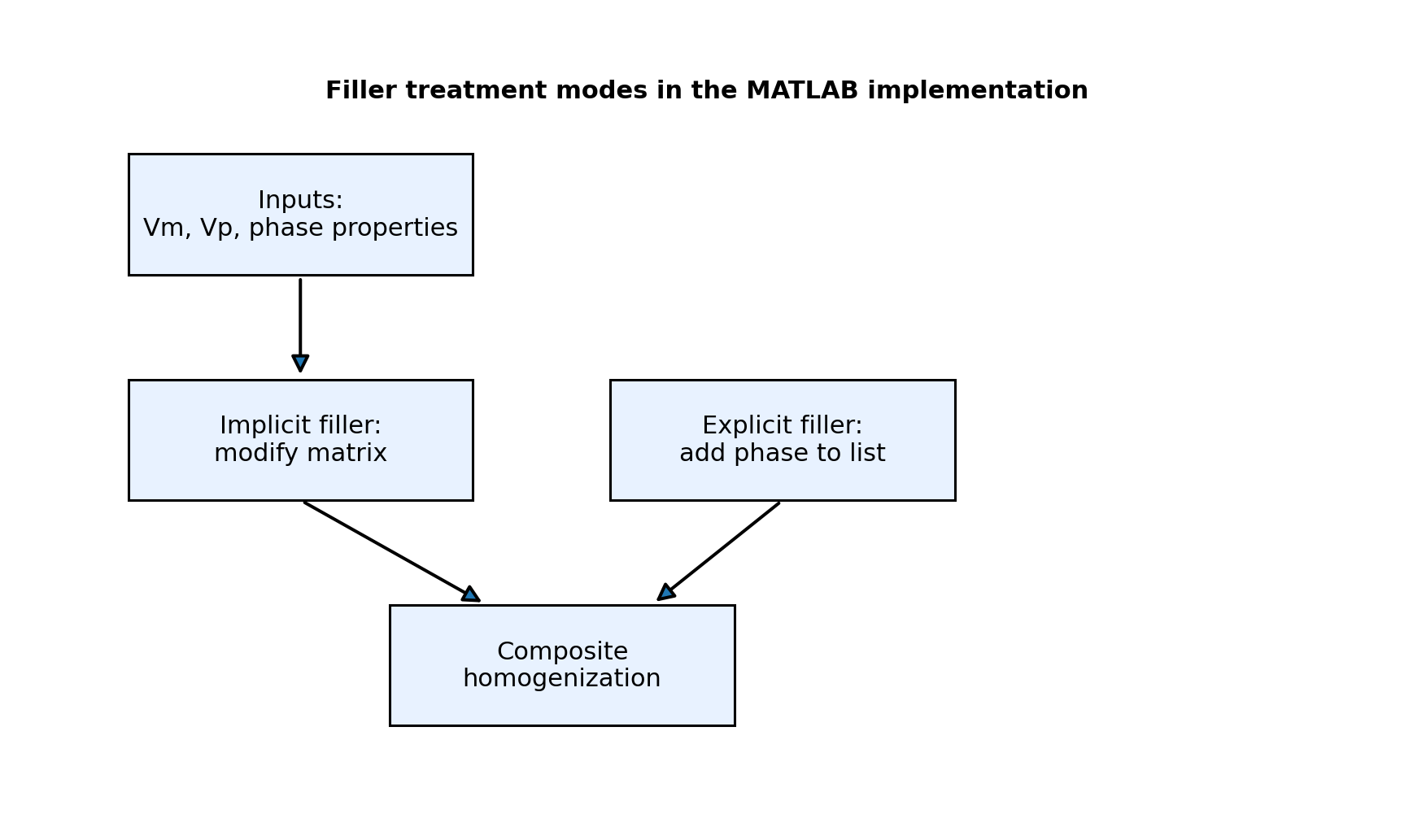
Figure V-II-S4-4. Implicit and explicit filler treatment modes. The implicit branch modifies the resin properties; the explicit branch adds filler as a separate homogenized phase.
4.5 Hybrid Fiber and Hybrid Tow Formulation
Hybrid composites contain two or more reinforcement families. Examples include carbon/glass hybrids, carbon/aramid hybrids, woven/braided hybrids, and fabrics containing binder or stitching yarns. The high-level hybrid stiffness relation can be written as
Meaning, notation and theory source
Definitions and derivation: 4.5 Hybrid Fiber and Hybrid Tow Formulation
where is the number of reinforcement families, is the volume fraction of family , is its homogenized stiffness, and is the transformation operator associated with its orientation or textile path.
For a two-family hybrid tow in an aligned limit,
Meaning, notation and theory source
Definitions and derivation: 4.5 Hybrid Fiber and Hybrid Tow Formulation
with
Meaning, notation and theory source
Definitions and derivation: 4.5 Hybrid Fiber and Hybrid Tow Formulation
The same concept is used in textile systems by treating warp, weft, bias, binder, or stitched reinforcements as separate reinforcement families with architecture-dependent weighting.
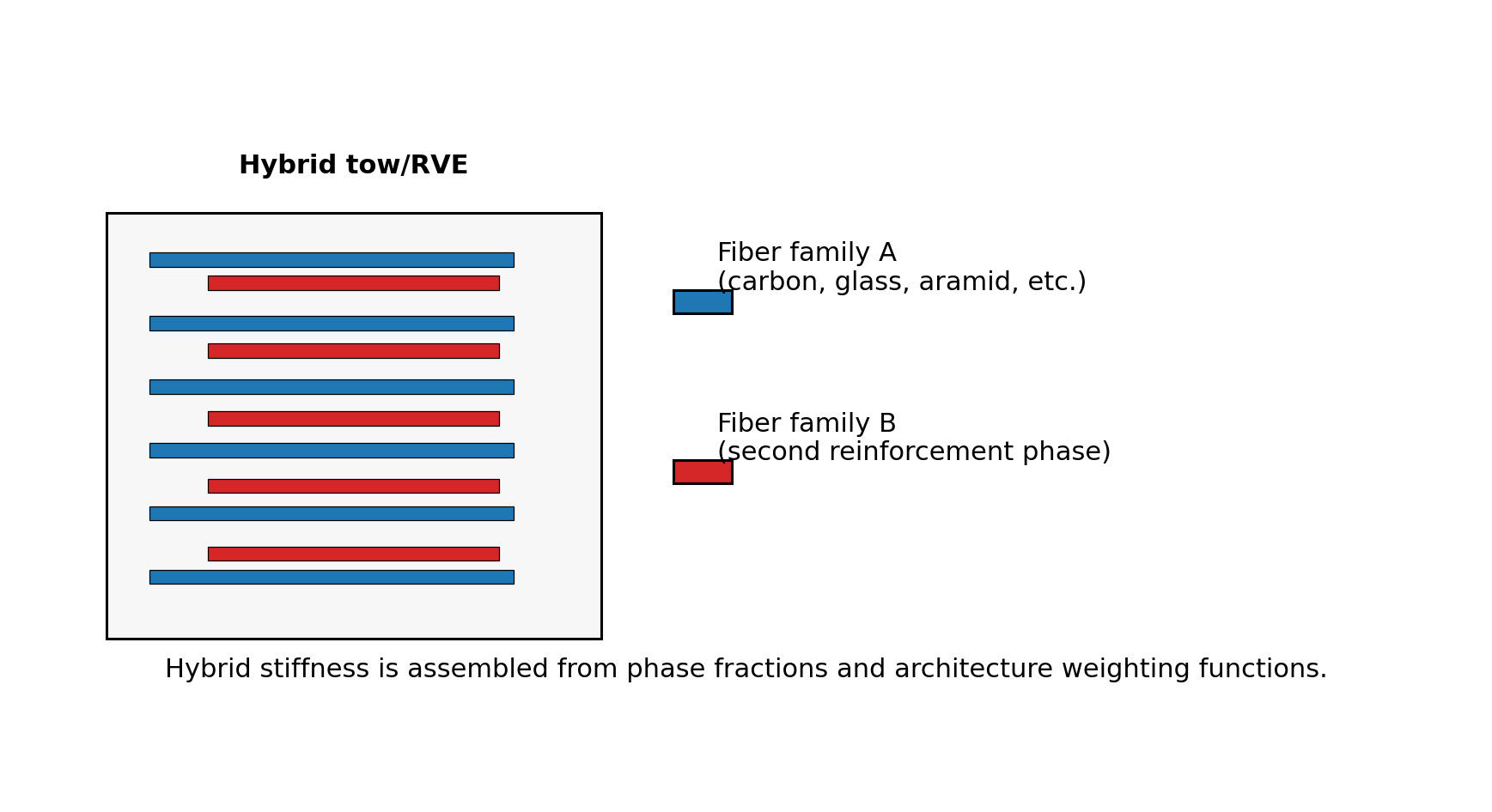
Figure V-II-S4-2. Hybrid fiber/tow representative volume element. Different reinforcement families are assembled using phase fractions and architecture-dependent weighting.
4.6 Void Phase Approximation
Voids are treated as a near-zero-stiffness phase or through property knockdown factors. The explicit void stiffness is represented by
Meaning, notation and theory source
which avoids singular numerical operations while preserving the strong softening effect of porosity. A first-order stiffness reduction can be written as
Meaning, notation and theory source
where is the void-free effective stiffness and is a void sensitivity factor. In engineering use, is larger for transverse and shear properties than for longitudinal fiber-dominated properties.
For density, the void contribution is negligible,
Meaning, notation and theory source
Voids also reduce thermal conductivity by interrupting heat-transfer paths,
Meaning, notation and theory source
where is direction dependent.
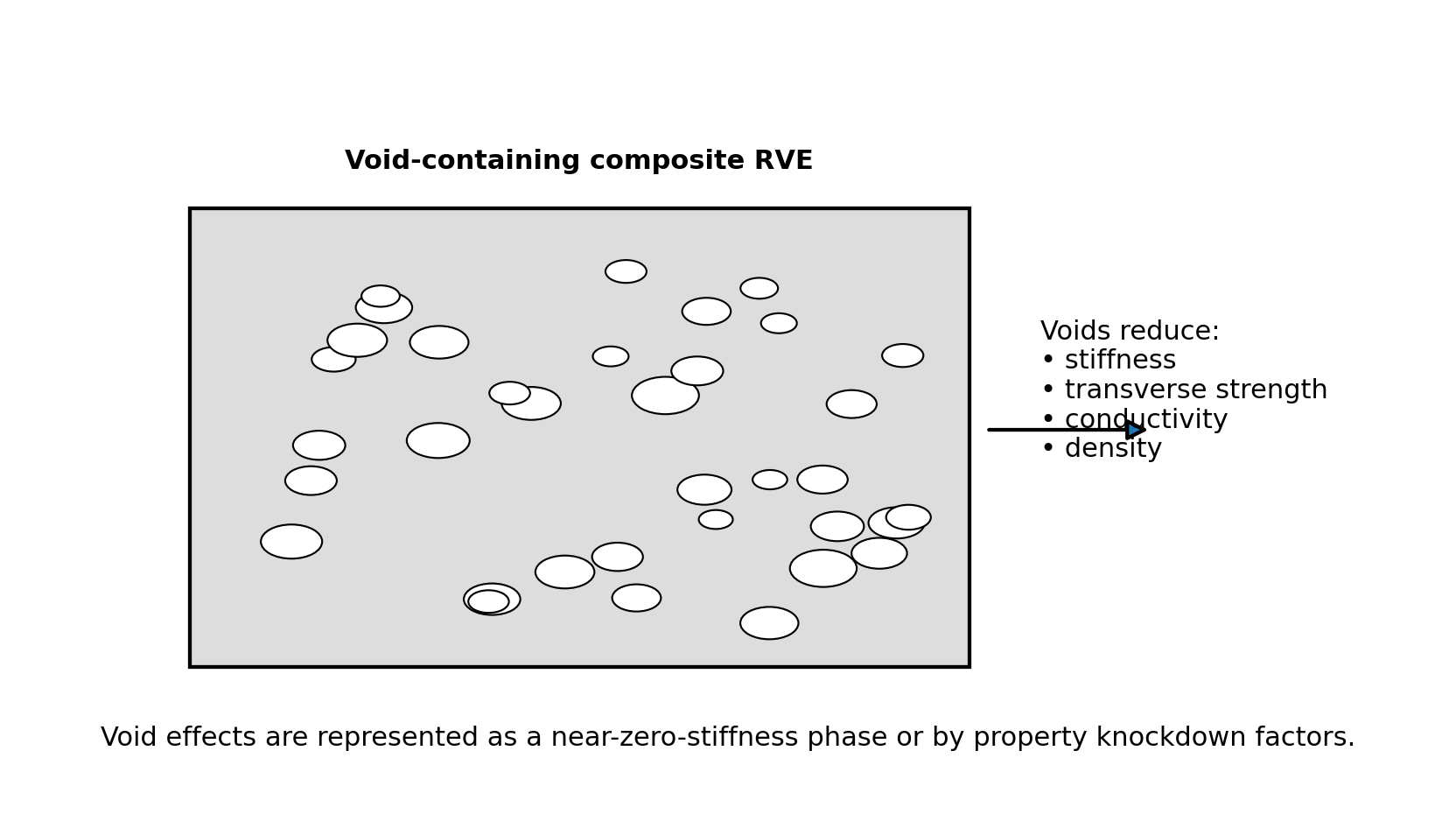
Figure V-II-S4-3. Void-containing composite RVE. Voids reduce stiffness, density, transverse strength, and effective conductivity.
4.7 Filled Matrix Density, Heat Capacity, and Conductivity
The filled matrix density follows direct volume averaging,
Meaning, notation and theory source
Definitions and derivation: 4.7 Filled Matrix Density, Heat Capacity, and Conductivity
The filled matrix specific heat is computed from volumetric heat capacity,
Meaning, notation and theory source
Definitions and derivation: 4.7 Filled Matrix Density, Heat Capacity, and Conductivity
For approximately spherical filler particles, the filled-matrix thermal conductivity is estimated as
Meaning, notation and theory source
Definitions and derivation: 4.7 Filled Matrix Density, Heat Capacity, and Conductivity
where
Meaning, notation and theory source
Definitions and derivation: 4.7 Filled Matrix Density, Heat Capacity, and Conductivity
These equations are consistent with the mechanical filled-matrix treatment and provide an efficient way to introduce filler effects into coupled thermomechanical analysis.
4.8 Effective Phase List Used by the solver Model
Meaning, notation and theory source
Definitions and derivation: 4.8 Effective Phase List Used by the solver Model
When filler is explicit, the matrix-like properties are built from matrix, filler, and void fractions only for engineering approximation of matrix-dominated behavior:
Meaning, notation and theory source
Definitions and derivation: 4.8 Effective Phase List Used by the solver Model
This keeps the Workbench data path compact while retaining the ability to account for particle and void effects.
4.10 Directional Dilute-Porosity Correction
The preferred void model separates dense-solid homogenization from porosity degradation. Fiber, matrix, and filler fractions are first normalized over the solid fraction . The fully dense composite is calculated first, avoiding the excessive sensitivity produced when a near-zero-stiffness void is inserted directly into a transverse Reuss-type relation.
Each property group then receives its own calibrated degradation factor:
Meaning, notation and theory source
Definitions and derivation: 4.10 Directional Dilute-Porosity Correction
| Property group | Default coefficient | Effect at 1% void |
|---|---|---|
Longitudinal modulus, E1 | 1.0 | approximately 1% reduction |
Transverse moduli, E2/E3 | 3.0 | approximately 3% reduction |
Shear moduli, G12/G13/G23 | 3.5 | approximately 3.5% reduction |
Longitudinal strengths, Xt/Xc | 2.0 | approximately 2% reduction |
| Transverse strengths | 6.0 | approximately 6% reduction |
| Shear strengths | 5.0 | approximately 5% reduction |
| Thermal conductivity | 1.5 | approximately 1.5% reduction |
Longitudinal stiffness is therefore less sensitive than transverse
and shear stiffness, while effective strengths receive their own
directional factors before failure evaluation and material export. A
legacy explicit near-zero-stiffness void phase remains available for
comparison. Setting void_phase_enabled_flag to zero forces
the global void fraction to zero. The applied factors are returned as
diagnostics for calibration and verification.
After porosity correction, the model continues to constituent-limit recovery, then rebuilds the dependent stiffness, compliance and output properties. The general porosity and multiphase bounds are supported by References [1]–[6] below.
4.11 Applicability and Limitations
The filled-matrix and hybrid phase models are intended for engineering screening, Workbench deployment, and finite-element material-card generation. The implicit filler model is most appropriate for fine particles at moderate loading, while the explicit phase model is preferred for high filler fraction, large property contrast, non-spherical filler, or systems where filler affects transport properties strongly.
Void modeling is intentionally conservative and should be calibrated against measured porosity/property data when used for qualification or acceptance. The current formulation does not resolve local stress concentrations around individual voids and does not replace a full finite-element RVE when local failure initiation near pores is of interest.
References
[1] R. M. Christensen, Mechanics of Composite Materials,
Wiley, 1979.
[2] T. Mura, Micromechanics of Defects in Solids, 2nd ed.,
Martinus Nijhoff, 1987.
[3] G. J. Dvorak, Micromechanics of Composite Materials,
Springer, 2013.
[4] S. Torquato, Random Heterogeneous Materials: Microstructure and
Macroscopic Properties, Springer, 2002.
[5] J. C. Halpin and J. L. Kardos, “The Halpin–Tsai equations: A
review,” Polymer Engineering and Science, 16, 344–352,
1976.
[6] Z. Hashin and S. Shtrikman, “A variational approach to the theory of
the elastic behaviour of multiphase materials,” Journal of the
Mechanics and Physics of Solids, 11, 127–140, 1963.
[7] G. P. Tandon and G. J. Weng, “The effect of aspect ratio of
inclusions on the elastic properties of unidirectionally aligned
composites,” Polymer Composites, 5, 327–333, 1984.
[8] R. M. Jones, Mechanics of Composite Materials, 2nd ed.,
Taylor & Francis, 1999.
3.10 Effective Density and Specific Heat
Volume II – Section 5: Effective Density and Specific Heat Capacity
5.1 Purpose and Scope
This section documents the high-level theory used in the solver micromechanics model to predict effective density and effective specific heat capacity for continuous, discontinuous, woven, hybrid, filler-reinforced, and void-containing composite materials. These quantities are thermophysical properties rather than stiffness properties; therefore, the governing equations are based primarily on conservation of mass and conservation of thermal energy rather than strain-concentration tensors. The model treats density and heat capacity as phase-averaged quantities that are evaluated after the phase volume fractions have been normalized.
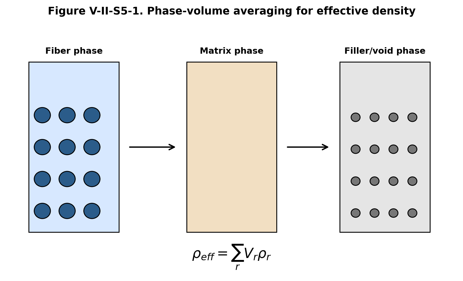
Figure V-II-S5-1. Phase-volume averaging for effective density.
5.2 Phase Definitions and Volume Constraint
The model considers up to four phase classes: fiber, matrix, filler, and void. The phase set is denoted by
Meaning, notation and theory source
Definitions and derivation: 5.2 Phase Definitions and Volume Constraint
where the subscripts represent fiber, matrix, particle/filler, and void, respectively. The normalized phase volume fractions satisfy
Meaning, notation and theory source
Definitions and derivation: 5.2 Phase Definitions and Volume Constraint
For the current Workbench, the filler volume may be treated either explicitly as a separate phase or implicitly as a modification to the matrix. When filler is treated explicitly, the global filler volume fraction is computed from the filler fraction inside the resin-rich phase. When filler is treated implicitly, the matrix density and matrix heat capacity are first modified and then used as effective matrix values in the remaining calculations.
5.3 Effective Density
Density is mass per unit volume. The total mass of the representative volume element is the sum of the phase masses:
Meaning, notation and theory source
For a phase volume and density , the phase mass is
Meaning, notation and theory source
The effective density is therefore
Meaning, notation and theory source
For the fiber–matrix–filler–void system used by the solver model,
Meaning, notation and theory source
The void density is taken to be a very small positive value in the implementation to avoid numerical singularities. For most engineering applications, the void contribution to density is negligible and Eq. (5.6) reduces to the weighted average of the solid phases.
5.4 Explicit and Implicit Filler Treatments
For explicit filler treatment, the filler phase appears directly in Eq. (5.6). The model uses the global phase fractions
Meaning, notation and theory source
Definitions and derivation: 5.4 Explicit and Implicit Filler Treatments
and the corresponding densities
Meaning, notation and theory source
Definitions and derivation: 5.4 Explicit and Implicit Filler Treatments
For implicit filler treatment, the filled matrix density is computed first:
Meaning, notation and theory source
Definitions and derivation: 5.4 Explicit and Implicit Filler Treatments
where is the filler volume fraction within the resin phase. The effective density then becomes
Meaning, notation and theory source
Definitions and derivation: 5.4 Explicit and Implicit Filler Treatments
This distinction is important because the same physical filler can be represented either as a separate phase in the homogenization list or as a modified matrix property.
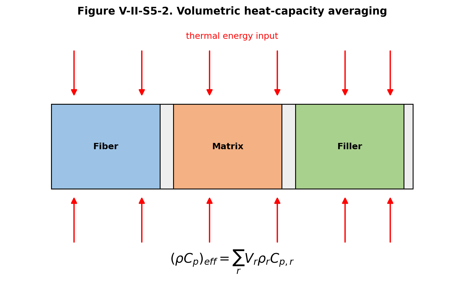
Figure V-II-S5-2. Volumetric heat-capacity averaging.
5.5 Effective Volumetric Heat Capacity
Specific heat capacity is defined per unit mass, while heat storage in a composite representative volume element is naturally additive per unit volume. For a uniform temperature change , the heat stored in phase is
Meaning, notation and theory source
Definitions and derivation: 5.5 Effective Volumetric Heat Capacity
The total heat stored in the RVE is
Meaning, notation and theory source
Definitions and derivation: 5.5 Effective Volumetric Heat Capacity
The effective volumetric heat capacity is therefore
Meaning, notation and theory source
Definitions and derivation: 5.5 Effective Volumetric Heat Capacity
The effective mass-specific heat capacity is obtained by dividing by the effective density:
Meaning, notation and theory source
Definitions and derivation: 5.5 Effective Volumetric Heat Capacity
For fiber, matrix, filler, and void phases,
Meaning, notation and theory source
Definitions and derivation: 5.5 Effective Volumetric Heat Capacity
In most composite analyses the void term is negligible; however, it is retained in the code for consistency with the general multiphase framework.
5.6 Filled-Matrix Heat Capacity
For implicit filler treatment, the filled-matrix volumetric heat capacity is
Meaning, notation and theory source
The filled-matrix specific heat is then
Meaning, notation and theory source
This is the form used when the filler is not included as an explicit phase in the global phase list.
5.7 Textile and Fabric Composite Considerations
For woven and stitched fabric composites, density and specific heat are not strongly affected by tow crimp or interlacing in the same way as stiffness. The primary dependence is through the phase volume fractions. However, the fabric architecture affects the final phase fractions because warp, weft, stitch, binder, and matrix-rich regions occupy different portions of the unit cell. A textile RVE may be represented by
Meaning, notation and theory source
Definitions and derivation: 5.7 Textile and Fabric Composite Considerations
The corresponding effective density is
Meaning, notation and theory source
Definitions and derivation: 5.7 Textile and Fabric Composite Considerations
If the warp and weft tows are made from the same constituent materials and use the same tow fiber volume fraction, the textile density reduces to the phase-averaged expression of Eq. (5.6). If different tow systems are used, Eq. (5.19) provides the appropriate hybrid-fabric form.
5.10 Verification Checks
The density and heat-capacity modules are verified using limiting and conservation checks. If all phases have the same density, then
Meaning, notation and theory source
If the fiber volume fraction vanishes and the filler is disabled, then
Meaning, notation and theory source
If the composite contains only fiber, then
Meaning, notation and theory source
These limiting checks are useful because density and heat capacity should be exact under phase averaging and should not depend on stiffness-model selection.
5.11 References
- R. M. Jones, Mechanics of Composite Materials, 2nd ed., Taylor & Francis, 1999.
- T. Mura, Micromechanics of Defects in Solids, 2nd ed., Martinus Nijhoff, 1987.
- G. J. Dvorak, Micromechanics of Composite Materials, Springer, 2013.
- C. C. Chamis, “Simplified composite micromechanics equations for hygral, thermal and mechanical properties,” SAMPE Quarterly, 15, 14–23, 1983.
- R. M. Christensen, Mechanics of Composite Materials, Wiley, 1979.
- S. Torquato, Random Heterogeneous Materials: Microstructure and Macroscopic Properties, Springer, 2002.
- N. K. Naik, Woven Fabric Composites, Technomic, 1994.
- D. Hull and T. W. Clyne, An Introduction to Composite Materials, Cambridge University Press, 1996.
3.11 Orthotropic Thermophysical Property Assembly
Volume II - Section 8
Orthotropic Thermophysical Property Assembly and Finite Element Material Definition
8.1 Purpose and Scope
This section describes the final assembly stage used by the Workbench solver micromechanics model to collect the mechanical and thermophysical predictions developed in the preceding sections of Volume II. The goal is to transform the homogenized composite response into a practical engineering material definition suitable for finite element analysis. The assembled output contains orthotropic elastic constants, density, coefficient of thermal expansion, thermal conductivity, and specific heat capacity.
The assembly operation is not a separate micromechanics theory by itself. Rather, it is the final bookkeeping and constitutive closure step that ensures all predicted properties are placed into consistent material directions and exported through the same data structures used by Workbench and Abaqus.
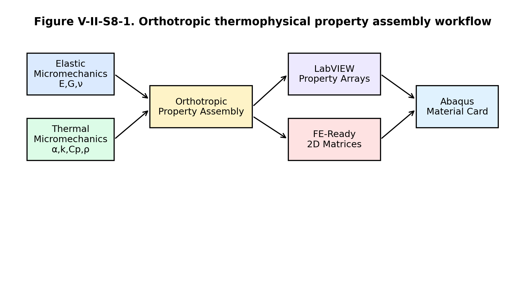
Figure V-II-S8-1. Orthotropic thermophysical property assembly workflow.
8.2 Effective Property Set
The final orthotropic property set is written as
Meaning, notation and theory source
Here, are the orthotropic Young’s moduli, are the orthotropic shear moduli, are the major Poisson ratios, is the effective density, are the coefficients of thermal expansion, are the principal thermal conductivities, and is the effective specific heat capacity.
The model stores the same assembled property set in the effective properties
Meaning, notation and theory source
This duplication is intentional. The orthotropic vector is used directly for engineering review, while the effective-property vector provides a generic interface for downstream software modules.
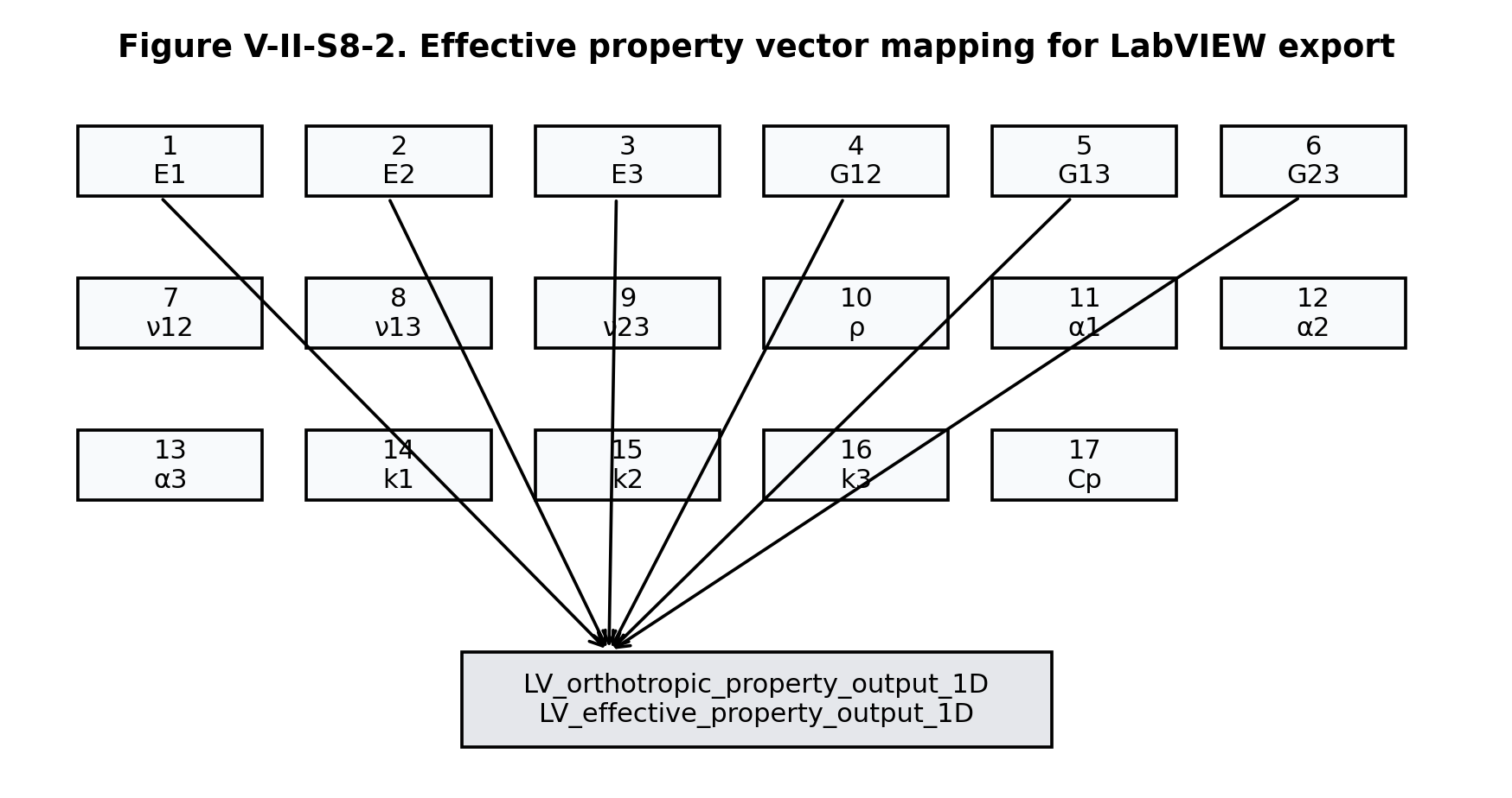
Figure V-II-S8-2. Effective property vector mapping for Workbench export.
8.3 Orthotropic Compliance Matrix
For finite element use, the orthotropic engineering constants are first assembled into the compliance matrix
Meaning, notation and theory source
Definitions and derivation: 8.3 Orthotropic Compliance Matrix
The stiffness matrix used for anisotropic finite element export is obtained by inversion,
Meaning, notation and theory source
Definitions and derivation: 8.3 Orthotropic Compliance Matrix
In the solver implementation this matrix is returned as both an orthotropic FE stiffness matrix and an anisotropic FE stiffness matrix. The orthotropic matrix is the symmetric stiffness constructed from engineering constants. The anisotropic matrix is the same matrix in the present model unless additional coupling terms are introduced by future orientation, damage, or transformation modules.
8.4 Thermoelastic Constitutive Form
The coupled orthotropic thermoelastic stress-strain relation is
Meaning, notation and theory source
Definitions and derivation: 8.4 Thermoelastic Constitutive Form
where
Meaning, notation and theory source
Definitions and derivation: 8.4 Thermoelastic Constitutive Form
For finite element applications, the thermal strain vector is
Meaning, notation and theory source
Definitions and derivation: 8.4 Thermoelastic Constitutive Form
The mechanical strain used in the constitutive update is therefore
Meaning, notation and theory source
Definitions and derivation: 8.4 Thermoelastic Constitutive Form
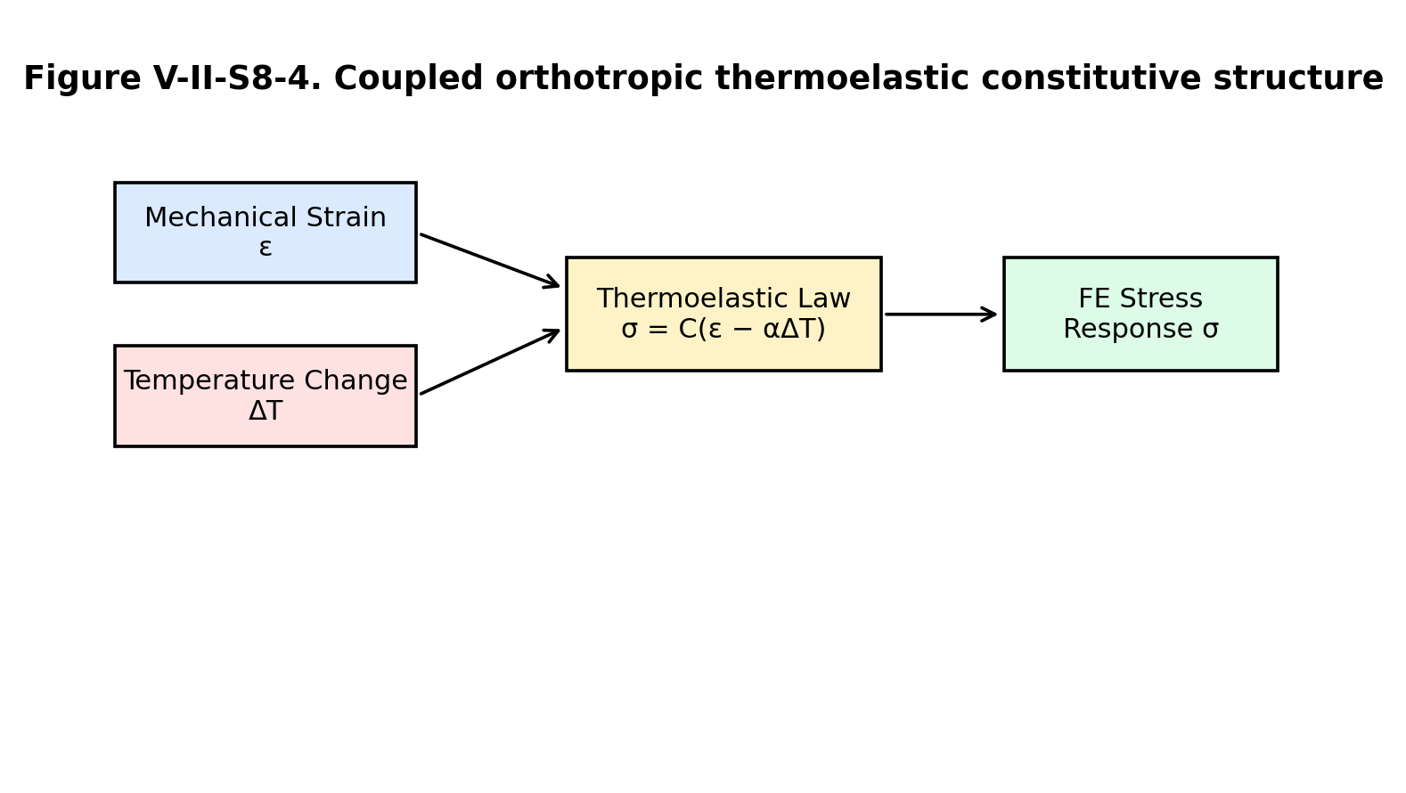
Figure V-II-S8-4. Coupled orthotropic thermoelastic constitutive structure.
8.5 Density and Heat Capacity Closure
The density and specific heat terms are scalar quantities in the finite element material definition. The effective density used in the FE card is
Meaning, notation and theory source
Definitions and derivation: 8.5 Density and Heat Capacity Closure
The effective specific heat is exported as
Meaning, notation and theory source
Definitions and derivation: 8.5 Density and Heat Capacity Closure
These values should be interpreted as homogenized continuum properties per unit mass of the equivalent composite material. In coupled thermal analyses, the volumetric heat capacity is
Meaning, notation and theory source
Definitions and derivation: 8.5 Density and Heat Capacity Closure
8.6 Thermal Conductivity Tensor
The orthotropic thermal conductivity matrix is assembled as
Meaning, notation and theory source
The corresponding heat-flux equation is Fourier’s law,
Meaning, notation and theory source
For an orthotropic material aligned with the finite element material coordinate system, the conductivity values are exported directly as , , and . If a global material orientation is applied in the structural model, the finite element solver performs the required transformation through the assigned material orientation.
8.8 Abaqus Material Definition
The assembled material properties are written to the single Workbench string variable
Meaning, notation and theory source
For an orthotropic engineering-constant definition, the basic Abaqus elastic card is
*MATERIAL, NAME=MICROMECHANICS_COMPOSITE
*ELASTIC, TYPE=ENGINEERING CONSTANTS
E1, E2, E3, NU12, NU13, NU23, G12, G13, G23
The thermophysical extension appends
*DENSITY
rho_eff
*EXPANSION, TYPE=ORTHO
alpha1_eff, alpha2_eff, alpha3_eff
*CONDUCTIVITY, TYPE=ORTHO
k1_eff, k2_eff, k3_eff
*SPECIFIC HEAT
Cp_eff
The anisotropic stiffness option exports the independent stiffness coefficients from the stiffness matrix rather than engineering constants.
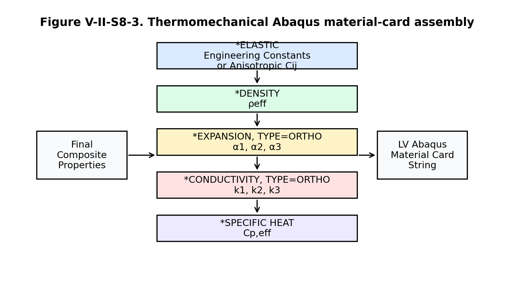
Figure V-II-S8-3. Thermomechanical Abaqus material-card assembly.
8.9 Verification Checks
The final assembly stage should satisfy the following basic consistency checks:
Meaning, notation and theory source
The compliance and stiffness matrices should be symmetric,
Meaning, notation and theory source
The stiffness matrix should be positive definite for a stable linear elastic material,
Meaning, notation and theory source
The thermal properties should also remain within physically reasonable bounds for the selected constituents and architecture.
8.11 Summary
The orthotropic thermophysical assembly step closes the multiscale modeling sequence by collecting all predicted properties into a consistent finite element material description. Mechanical constants are assembled into compliance and stiffness matrices. Density, thermal expansion, thermal conductivity, and specific heat are appended to complete the thermomechanical material definition. This final assembly enables direct use of the micromechanics results in Workbench workflows and Abaqus finite element simulations.
References
- R. M. Jones, Mechanics of Composite Materials, Taylor & Francis, 1999.
- G. J. Dvorak, Micromechanics of Composite Materials, Springer, 2013.
- T. Mura, Micromechanics of Defects in Solids, Martinus Nijhoff, 1987.
- Y. Benveniste, “A new approach to the application of Mori-Tanaka’s theory in composite materials,” Mechanics of Materials, 6, 147-157, 1987.
- T.-W. Chou, Microstructural Design of Fiber Composites, Cambridge University Press, 1992.
- Dassault Systemes, Abaqus Analysis User’s Guide, material definitions for engineering constants, expansion, conductivity, density, and specific heat.
3.12 Verification, Validation, and References
Volume II - Section 9
Verification, Validation, and References for Textile and Thermophysical Micromechanics
9.1 Purpose and Scope
This section summarizes the recommended verification and validation methodology for the textile, hybrid, filled-matrix, and thermophysical property models described in Volume II. The purpose is to document how the implemented solver model should be checked against mathematical limits, engineering benchmarks, and published reference data before the output is used for finite-element material definition or Workbench-based design workflows.
The verification process confirms that the implementation obeys expected limiting behavior, conservation laws, tensor symmetry, and material-property bounds. The validation process compares the model predictions with independent data, such as coupon-level textile composite measurements, constituent mixture data, thermophysical test data, and published micromechanics benchmarks.
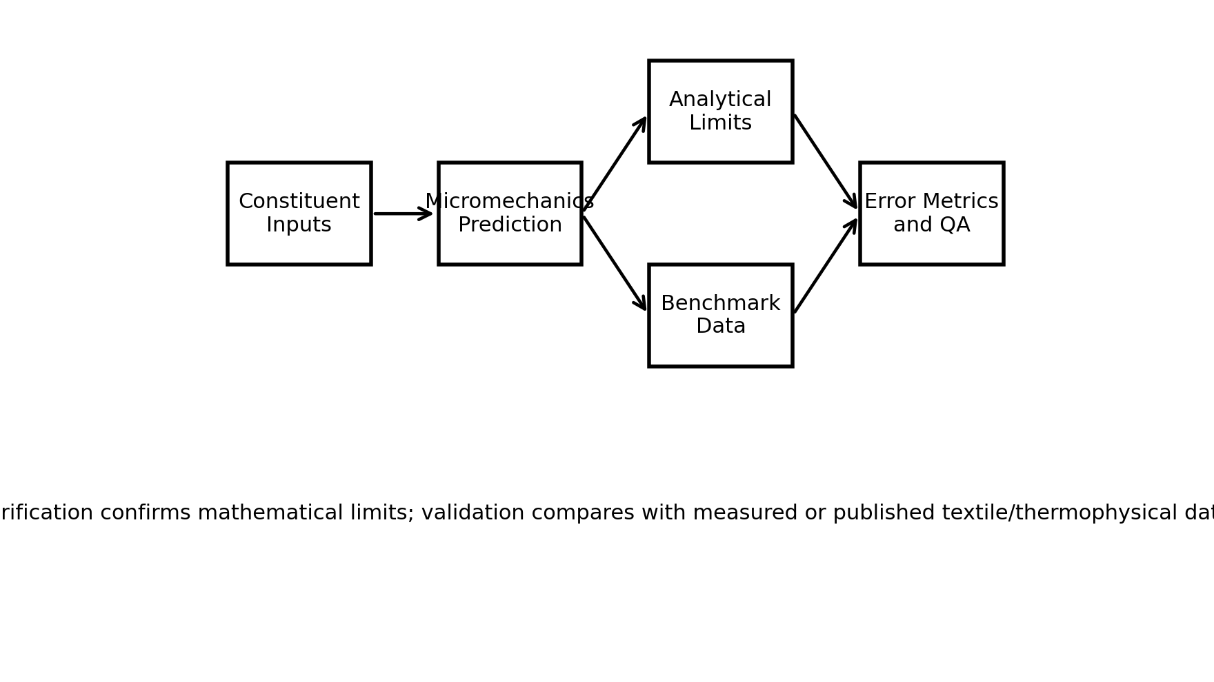
Figure V-II-S9-1. Verification and validation workflow for the textile and thermophysical micromechanics modules.
9.2 Verification Philosophy
Verification asks whether the equations have been implemented correctly. For the present model, verification is performed by exercising the code under controlled limiting cases. The general verification requirement is written as
Meaning, notation and theory source
where is the vector of input variables and is the predicted effective property vector. For Volume II, the property vector includes elastic, density, specific heat, thermal conductivity, and thermal expansion terms,
Meaning, notation and theory source
The normalized verification error for a scalar property is
Meaning, notation and theory source
For a vector of properties, the global relative error is
Meaning, notation and theory source
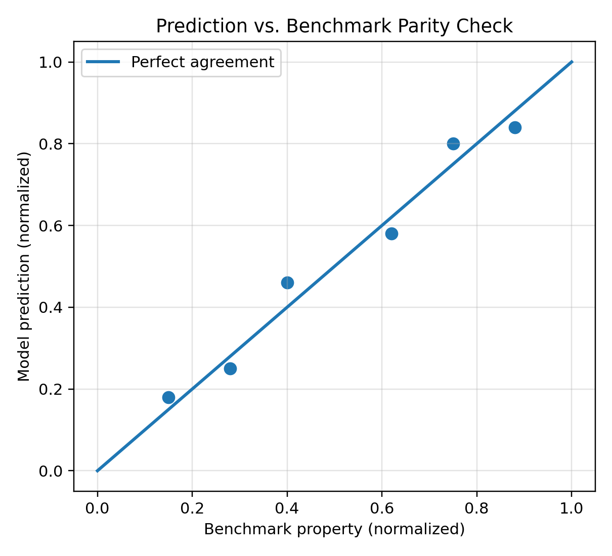
Figure V-II-S9-2. Generic parity plot used to compare model predictions against benchmark data.
9.3 Limiting-Case Checks
The most important verification cases are the limiting conditions that recover known material behavior. When the fiber volume fraction approaches zero, the composite must recover the filled or neat matrix response,
Meaning, notation and theory source
When the filler volume fraction approaches zero, the filled matrix must reduce to the neat resin,
Meaning, notation and theory source
When the void volume fraction approaches zero, the void-corrected property must reduce to the non-voided composite property,
Meaning, notation and theory source
For a balanced woven composite with equal warp and weft fractions and identical tow properties, the in-plane moduli should approach one another,
Meaning, notation and theory source
If the crimp amplitude approaches zero, the crimp knockdown should approach unity,
Meaning, notation and theory source
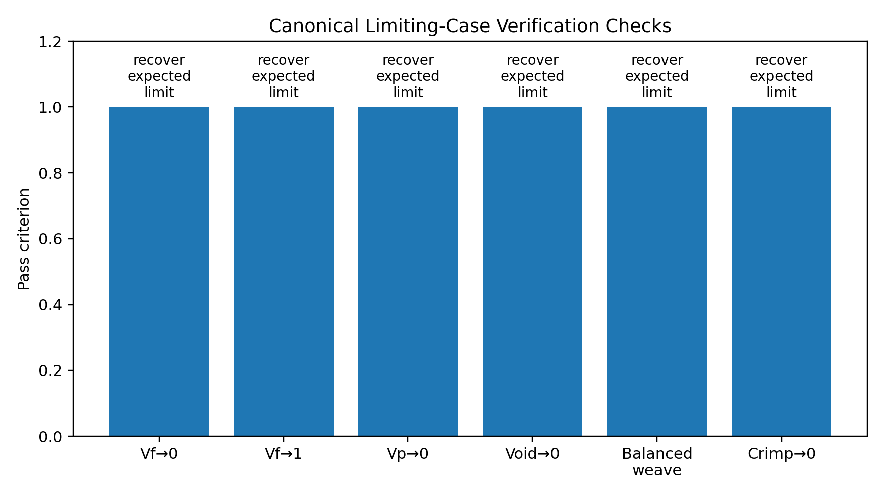
Figure V-II-S9-3. Limiting-case checks used to verify textile and thermophysical model behavior.
9.4 Thermophysical Property Verification
Density is verified using conservation of mass. The implemented effective density must equal the volume-weighted sum of all active phases,
Meaning, notation and theory source
Definitions and derivation: 9.4 Thermophysical Property Verification
The specific heat is verified by checking conservation of thermal energy,
Meaning, notation and theory source
Definitions and derivation: 9.4 Thermophysical Property Verification
The longitudinal and transverse thermal conductivity predictions should remain bounded by the parallel and series estimates,
Meaning, notation and theory source
Definitions and derivation: 9.4 Thermophysical Property Verification
The CTE prediction should approach the matrix expansion coefficient as reinforcement volume fraction approaches zero,
Meaning, notation and theory source
Definitions and derivation: 9.4 Thermophysical Property Verification
For a stiff, low-CTE fiber in a polymer matrix, the axial CTE should typically decrease as fiber volume fraction increases,
Meaning, notation and theory source
Definitions and derivation: 9.4 Thermophysical Property Verification
9.5 Textile Architecture Verification
Architecture factors should produce physically meaningful trends. The architecture-corrected fabric stiffness may be expressed schematically as
Meaning, notation and theory source
Definitions and derivation: 9.5 Textile Architecture Verification
and
Meaning, notation and theory source
Definitions and derivation: 9.5 Textile Architecture Verification
For an unbalanced fabric, increasing the warp fraction should increase and reduce relative to the balanced case,
Meaning, notation and theory source
Definitions and derivation: 9.5 Textile Architecture Verification
The in-plane shear modulus is penalized by interlacing and crimp corrections,
Meaning, notation and theory source
Definitions and derivation: 9.5 Textile Architecture Verification
For low-interlacing satin architectures, the interlacing penalty should be weaker than for plain weave,
Meaning, notation and theory source
Definitions and derivation: 9.5 Textile Architecture Verification
For non-crimp fabric, the crimp factor should be close to unity, subject to any stitching knockdown,
Meaning, notation and theory source
Definitions and derivation: 9.5 Textile Architecture Verification
9.6 Validation Against Benchmark Data
Validation compares model predictions against experimental or published benchmark values. For each benchmark property , the percentage error is
Meaning, notation and theory source
Definitions and derivation: 9.6 Validation Against Benchmark Data
For a set of properties, the mean absolute percentage error is
Meaning, notation and theory source
Definitions and derivation: 9.6 Validation Against Benchmark Data
A root-mean-square normalized error may also be used,
Meaning, notation and theory source
Definitions and derivation: 9.6 Validation Against Benchmark Data
The recommended benchmark classes are summarized in Figure V-II-S9-4.
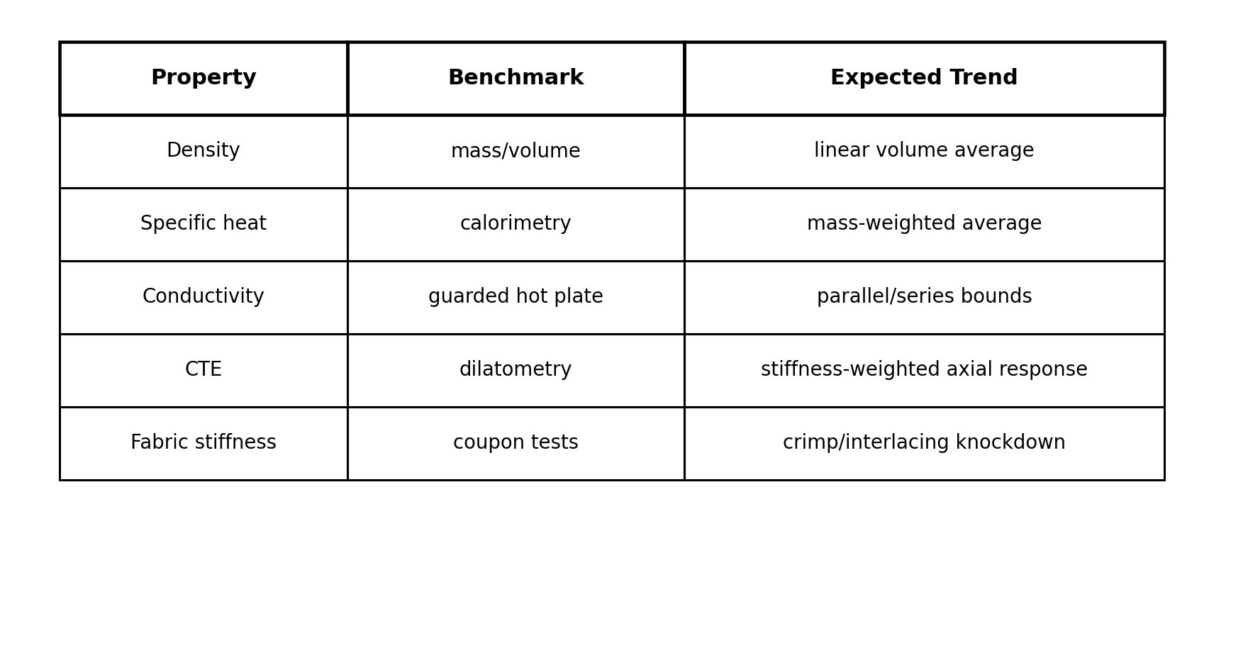
Figure V-II-S9-4. Recommended validation matrix for Volume II textile and thermophysical predictions.
9.7 Recommended Validation Cases
The following validation cases are recommended for the current implementation:
- Balanced plain-weave carbon/epoxy: verify , CTE balance, and crimp knockdown.
- Unbalanced woven glass/epoxy: verify sensitivity to warp/weft fraction.
- Satin carbon/epoxy: verify reduced interlacing penalty relative to plain weave.
- Non-crimp biaxial fabric: verify near-straight tow response with stitch knockdown.
- Particle-filled epoxy: verify density, conductivity, and stiffness trends with filler volume fraction.
- Voided composite: verify monotonic reduction in stiffness and density with increasing void content.
- Thermal conductivity benchmark: compare , , and against parallel/series bounds and measured values.
- CTE benchmark: compare , , and against dilatometry data.
9.8 Numerical Stability Checks
The property extraction and finite-element export require positive stiffness and finite thermophysical outputs. The compliance matrix must be nonsingular,
Meaning, notation and theory source
The stiffness matrix should be symmetric,
Meaning, notation and theory source
The principal elastic moduli and shear moduli must be positive,
Meaning, notation and theory source
Thermophysical quantities must remain finite and physically meaningful,
Meaning, notation and theory source
These checks are particularly important when the model is embedded in Workbench, because inconsistent input data, excessive void fractions, or nonphysical constituent data can otherwise propagate into Abaqus material definitions.
9.10 References
Advani, S. G., and Tucker, C. L. III. 1987. The use of tensors to describe and predict fiber orientation in short fiber composites. Journal of Rheology, 31, 751-784.
Chamis, C. C. 1983. Simplified composite micromechanics equations for hygral, thermal and mechanical properties. SAMPE Quarterly, 15, 14-23.
Chou, T.-W. 1992. Microstructural Design of Fiber Composites. Cambridge University Press.
Daniel, I. M., and Ishai, O. 2006. Engineering Mechanics of Composite Materials. Oxford University Press.
Dvorak, G. J. 2013. Micromechanics of Composite Materials. Springer.
Ishikawa, T., and Chou, T.-W. 1982. Stiffness and strength behavior of woven fabric composites. Journal of Materials Science, 17, 3211-3220.
Jones, R. M. 1999. Mechanics of Composite Materials. Taylor & Francis.
Lomov, S. V., Ivanov, D. S., Verpoest, I., Zako, M., Kurashiki, T., Nakai, H., and Hirosawa, S. 2007. Meso-FE modelling of textile composites: Road map, data flow and algorithms. Composites Science and Technology, 67, 1870-1891.
Mura, T. 1987. Micromechanics of Defects in Solids. Martinus Nijhoff.
Naik, N. K. 1994. Woven fabric composites. Technomic Publishing.
Whitcomb, J. D. 1991. Three-dimensional stress analysis of plain weave composites. Composite Materials: Testing and Design, ASTM STP.
Chapter review
Pass the effective elastic tensor, density and directional expansion and transport properties with their coordinate convention. Retain separate provenance for each property family. A model calibrated for elastic stiffness is not automatically calibrated for thermal conductivity, diffusion or strength.
References and source sections
References are retained with the formulations they support. Software instructions describe implementation scope; a cited source does not establish independent validation of a CDS calculation.