Explore designs in CREATE and DISCOVER

Design exploration is most useful after the baseline can be reproduced. Decide which quantities are independent variables and which are held fixed, then identify the response represented by every axis and colour. A contour interpolates between evaluated points; making that contour smoother does not add information about designs that were never calculated.

CREATE now assembles a fixed workflow study with compatible database selectors, class filters and Favorites. The live composite renderer follows the chosen materials, microstructure and laminate. DISCOVER retains those records and adds comparisons and available solved plots; Workbench exposes the full inputs. Undo and Redo preserve reversible study edits.

7.1 From a starting recipe to a checked design

Build a connected starting point in CREATE

CREATE begins with fixed workflow blocks whose compatible database selectors unlock as dependencies are connected. Materials and laminate selection can provide alternative starting paths. Use the neighbouring class/type filter, search and Favorites to shorten a list; a laminate selection also narrows compatible exercises. Existing finds laminates containing the chosen materials; format selection reuses the layup with the selected material or Micro recipe and hides duplicate layup formats. Confirm every ply source before proceeding. Disabled downstream blocks identify missing prerequisites, while Undo and Redo allow reversible changes.

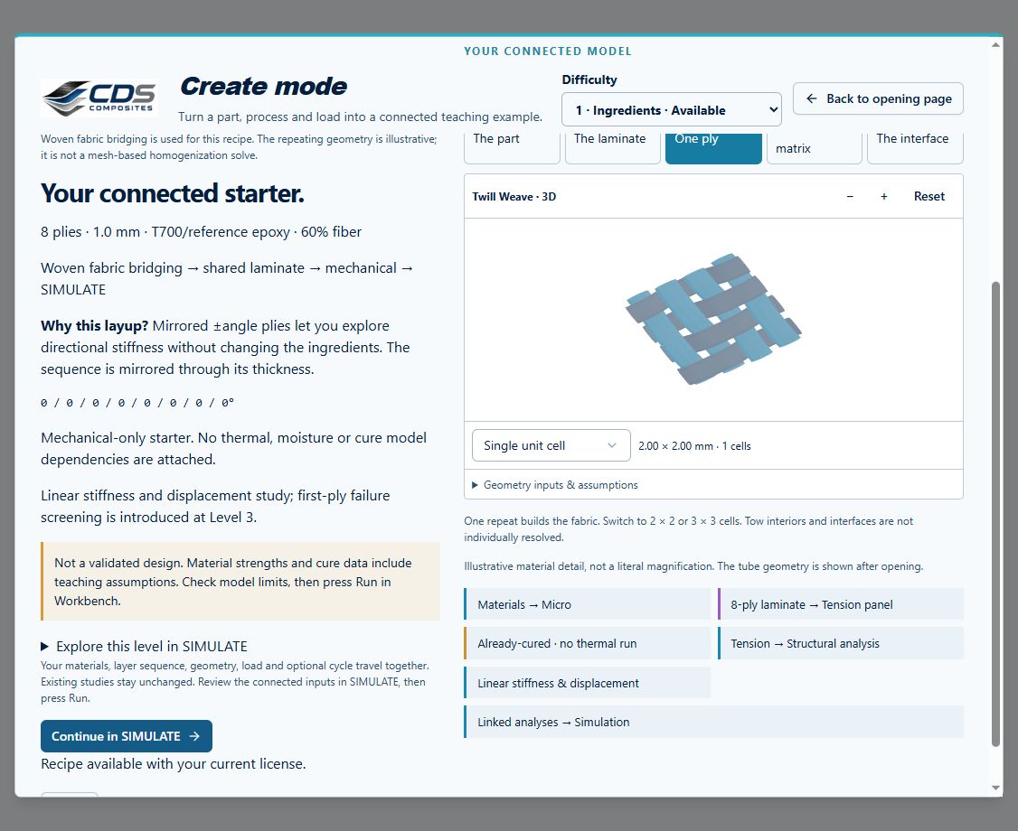
The live composite renderer now follows material, microstructure and laminate choices on a white background. Continuous zoom moves between laminate, ply and fiber/matrix scales without using zoom to explode the stack. Thermal, moisture and load callouts represent connected case inputs. Thermal and Mechanical selectors are classified by process or load type, and long lists provide filters. The fixed blocks retain their icons and selections while the renderer shows geometry detail. The older woven-fabric capture below illustrates the distinction between a visual architecture and a calculated result. Its connected starter contains eight plies with a total thickness of 1.0 mm and a stated fiber fraction of 60%. The interface identifies a mechanical-only, already-cured study: thermal, moisture and cure dependencies are not attached. Those values describe this particular teaching example, not requirements for every CREATE study. The yarn geometry helps explain the architecture, but is not a resolved mesh-based homogenization calculation.

Investigate the ingredients in DISCOVER

DISCOVER carries the connected CREATE study forward and provides an intermediate level of control before the full Workbench. It combines design-space exploration with available calculated temperature, stress and other result plots; run the applicable case before interpreting solved fields. Undo and Redo apply to reversible study edits. DISCOVER lets you relate the part to its laminate, individual ply, constituent materials and interface. Move between those views to understand which scale a property belongs to. For a controlled comparison, retain the original selection, change one available ingredient or architecture parameter, and inspect the corresponding response. A change in the geometry illustration is not, by itself, evidence of a change in predicted stiffness or strength; check the reported quantity and the model that produced it.

For woven materials, the unit-cell view exposes the repeating yarn arrangement. A tiled patch is useful for understanding repetition and orientation, but the displayed yarns do not establish that local tow interiors or interfaces have been solved. Keep the geometric explanation separate from the homogenized properties used by the downstream laminate. The fabric view in the laminate chapter provides a companion illustration.

Read a design-space map as a comparison

Before interpreting a two- or three-dimensional design-space plot, identify the two varied inputs, their bounds, the quantity represented by height or color, and any constraints applied to the candidates. Locate the baseline and compare it with a candidate that answers the original engineering question. A smooth surface or closely spaced contour levels can clarify the display, but they do not add evaluated designs or demonstrate numerical convergence. Increase the calculation’s sampling resolution, where supported, when testing whether a trend is adequately resolved.

Carry the selected candidate into the compatible SIMULATE workflow, inspect its linked records and run the required calculation. Check that its loads, material sources and dimensions are still the ones intended for comparison. Preserve both the baseline and the selected candidate, and describe the improvement together with the model’s limits. This closes the loop from guided exploration to a traceable study rather than treating a visually attractive point as a finished design.

7.2 Evaluate the complete composite structure.

Workflow / 03.5 Design

Choose a compatible released plate, cylinder, beam, section, joint or analytical study. Shared laminate inputs do not make every model combination valid.

Connected model layer

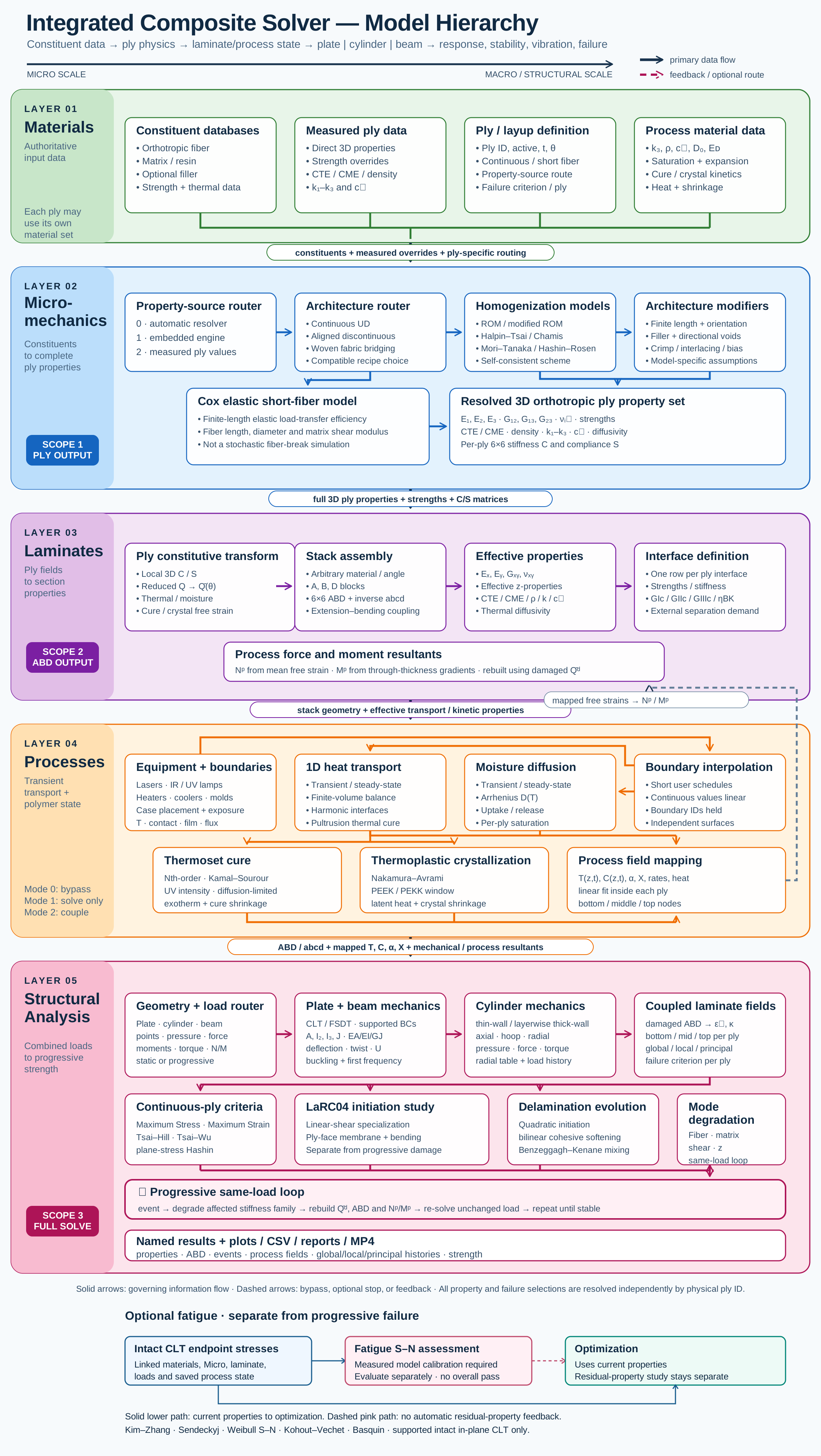
Structural analysis and design model map

Select a block to explore its theory or workflow. View the complete Model Map

Workbench path

Choose. Inspect. Refine.

01

▣

Select the case

Choose a simulation block and the run you want to study.

→

02

⌖

Inspect in Live Sim

See geometry, assignments and results together.

→

03

↻

Refine the model

Change geometry or selections and follow the downstream effect.

Open the complete block workflow guide ↗

Workbench exercise preview

02.10 · Three-point bending: span and stiffness

Level 3
IntermediateEst. 25 min

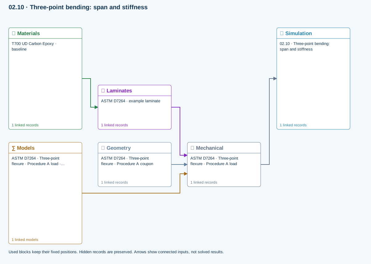
∑ Used models & submodels

Only models assigned to records used by this exercise are listed here. The full-layout option preserves the supplied starter records; no Workbench records are changed.

Euler–Bernoulli beam · Linear static · ASTM D7264 · Three-point flexure · Procedure A load

Beam bending uses effective laminate axial stiffness, the linked section geometry, support span and applied loading. Euler–Bernoulli deflection excludes transverse shear deformation, roller contact and indentation. Ply stress recovery for rectangular laminate coupons is separate from section-level beam stress recovery.

∑ Theory & assumptions

Data travelling between blocks

Materials → Laminates
Stored ply stiffness, strength, density and expansion properties.

Mechanical → Simulation
SIMULATION selects this case and its analysis model; the case owns its applicable cycle and input references.

Laminates → Mechanical
Ply angles and thicknesses, stiffness, mass and ply properties.

Geometry → Mechanical
Part shape and dimensions, thickness or section definition, and model-specific geometric inputs. Each selected case consumes only the dimensions its model supports.

Models → Mechanical
Applied model assignment: Euler–Bernoulli beam · Linear static. Model parameters and formulation are used by Mechanical.

Inspect specimen width, laminate thickness, support span and central force.

Models: Euler–Bernoulli beam · ASTM D7264-based

Study scope and limitations

Procedure A teaching setup. Transverse shear deformation, roller contact and indentation are excluded.

03.5 / Workflow focus

Connected engineering record

01

Plate and beam response

Use the released CLT/FSDT finite-plate or membrane/beam path with compatible dimensions, loads and supports. Buckling, modal and static bending are distinct study choices.

02

Cylinder formulations

Thin-wall membrane and layerwise thick-wall elasticity have different load and process limits. Donnell axial buckling is a separate thin-shell study with an explicit knockdown factor.

03

Sections and joints

Layerwise sections, lap joints and sandwich bending have their own geometry and interfaces. The analytical Volkersen / Goland–Reissner study is a separate identical-adherend elastic approximation.

04

Failure and notches

The five existing criteria support eligible CLT first-ply / progressive calculations. LaRC04 linear-shear initiation and calibrated open-hole strength are separate studies, not additional progressive choices.

05

Fatigue

S–N models predict life from calibrated data. Residual stiffness / strength requires independently fitted retention laws in its separate study; neither automatically changes optimization properties.

06

Creep, shape and uncertainty

Reference-state studies explore time response, prescribed-eigenstrain free release and bounded ABD sampling. Their scope, inputs and output handoffs are listed below.

07

Keep validation data connected

Run the selected Simulation after relevant edits. Review model assumptions, stale-result warnings, convergence and calibration before interpreting the result.

Use this workflow in Workbench: interactive Blocks, record selections and connection controls →

Connected model layer

Design · released model connections

Select a model family to follow its inputs, results, theory and exercise. All model families ↗

Follow the connections

Heat, moisture & manufacturing

Inputs

Material laws & boundary cycles

Roller radius, width, coating or metal properties, applied force and supported contact assumptions

Choose a model family

Transport & reaction

Results / handoff

History & compatible process fields

Contact footprint and pressure feeding applicable moving-process thermal and quality histories

Thermal starting point: add roller Geometry and a roller boundary for a contact study; the supplied die exercise does not contain a roller.

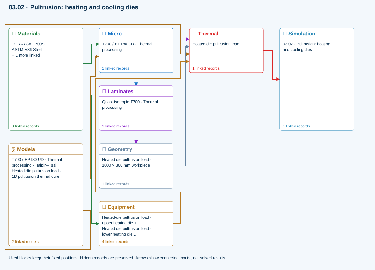
Rubber-covered roller contact

Bonded coating on a rigid core against a rigid flat. Geometry selects Infinite width (analytical plane strain) or Finite width (3D elastic contact with axial end spreading). Small deformation and optional prescribed sliding friction; no hyperelasticity or rolling resistance.

Model choices and Workbench location

Geometry → Rollers; Models → Roller contact

• Bonded-layer roller contact

7.3 Explore capacity and trade-offs without losing the assumptions.

04.11 / CDS User Guide

Practical operation of Response, failure envelopes, progressive failure, 2D/3D carpet plots, lamina/micro studies, laminate searches and saved optimization validation data.

06.1 Manuals · read online, preview or download →

Read the WB equations and limitations →

Workbench exercise preview

02.10 · Three-point bending: span and stiffness

Level 3
IntermediateEst. 25 min

∑ Used models & submodels

Only models assigned to records used by this exercise are listed here. The full-layout option preserves the supplied starter records; no Workbench records are changed.

Euler–Bernoulli beam · Linear static · ASTM D7264 · Three-point flexure · Procedure A load

Beam bending uses effective laminate axial stiffness, the linked section geometry, support span and applied loading. Euler–Bernoulli deflection excludes transverse shear deformation, roller contact and indentation. Ply stress recovery for rectangular laminate coupons is separate from section-level beam stress recovery.

∑ Theory & assumptions

Data travelling between blocks

Materials → Laminates
Stored ply stiffness, strength, density and expansion properties.

Mechanical → Simulation
SIMULATION selects this case and its analysis model; the case owns its applicable cycle and input references.

Laminates → Mechanical
Ply angles and thicknesses, stiffness, mass and ply properties.

Geometry → Mechanical
Part shape and dimensions, thickness or section definition, and model-specific geometric inputs. Each selected case consumes only the dimensions its model supports.

Models → Mechanical
Applied model assignment: Euler–Bernoulli beam · Linear static. Model parameters and formulation are used by Mechanical.

Inspect specimen width, laminate thickness, support span and central force.

Models: Euler–Bernoulli beam · ASTM D7264-based

Study scope and limitations

Procedure A teaching setup. Transverse shear deformation, roller contact and indentation are excluded.

01

Results controls and exports

Outputs keeps the selected Materials, Micro, Laminates, Thermal, Moisture, Structural or Optimization view. Table, Ashby, Bar and Line views share selection and property controls; physics-specific views add response, profile, field, failure and plot controls.

Step-by-step instructions · 5 steps

1. Select one record for inspection or Ctrl/Command-click and Shift-click compatible records for comparison. Folder and class filters narrow the rows without changing records.
2. Choose plotted properties, axes and classes, then use autoscale locks when a stable comparison range is required.
3. Right-click supported plots for markers, autoscale and image or data exports. Table export offers CSV, Excel, Word or PowerPoint where shown.
4. Use Inputs, Split, Outputs and pane expand controls to allocate space. Drag internal splitters between controls, plots and tables.
5. Treat missing, stale and not-assessed messages as result states; they are not zero values.

02

Optimization controls and saved studies

Optimize Inputs chooses Laminate, Lamina/Micro or Process mode. Each mode provides a study selector, objective, variables, bounds, constraints, search controls, plots, candidate actions and Save snapshot. Compatible favorites sort first in study and source selectors.

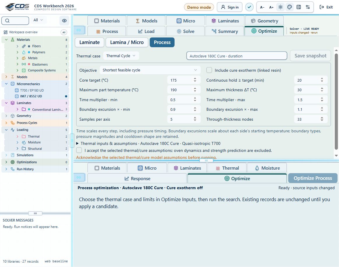
Step-by-step instructions · 5 steps

1. Select the mode and study, then resolve every readiness message before starting a search.
2. Set bounds and constraints in the displayed units; locks and unavailable variables explain what the active model permits.
3. Run or stop the search, inspect evaluated and feasible counts, convergence and the best candidate, then Apply or Create new only when enabled.
4. Name and save an optimization snapshot to preserve the study and download its CDS_DB. Open saved cases below Simulations and compare compatible cases.
5. Use New optimization to return to editable search controls. Saved optimization inputs remain read-only evidence.

03

High-ply-count optimization

Two core exercises start with 48 and 64 active plies for minimum-mass and fixed-count strength studies.

Step-by-step instructions · 3 steps

1. Run the baseline and confirm ply count, thickness, loads and strengths.
2. Follow the exercise angle set, symmetry, balance, search budget and seed. The released search supports 1–64 plies.
3. Compare seeds 42 and 43. Save the best feasible candidate, create its laminate separately and rerun structural analysis.

04

Explore a failure step and explain a hotspot

The slider above the progressive 2D plot is connected to its cursor. Drag either to inspect a saved step; the arrow controls jump between activations. The depth selector sits with the other plot controls.

Step-by-step instructions · 3 steps

1. Select the step and ply, then expand Explain selected hotspot for its criterion, mode, local stress and theory link.
2. Use the vertical Fiber, Matrix and Shear strip: gray means not activated, color means activated, and a gold outline marks a new activation at this step. Select a strip segment to inspect that ply.
3. Use the output expand control for more space and restore Split when returning to input editing.

05

Include delamination in progressive steps

The ordinary CLT progressive ramp degrades plies; it does not separate their interfaces. For supported coupled growth, choose Layerwise x-z plane strain and set Delamination model to Coupled growth.

Step-by-step instructions · 4 steps

1. Link finite Plate geometry and a laminate with complete 3D stiffness.
2. Supply calibrated interface stiffness, normal/shear strengths, fracture energies and BK exponent, plus ply strengths and load-step controls. No interface properties are inferred from a laminate name.
3. Run the linked simulation, then open Response → Progressive failure · plies + delamination.
4. Check mesh and step convergence and compare with the connected simulation-20 exercise and cohesive theory.

06

Optimization cases: Micro, Process and Laminate

Optimizations contains Micro, Process and Laminate subfolders. New saved cases retain the numerical study, all search variables and constraints, and a frozen archive of linked source records and process boundary schedules. Older snapshots remain readable but cannot recover source records that were never saved.

Step-by-step instructions · 4 steps

1. Configure and run the selected optimizer, name the case and choose Save snapshot. The case is added to its mode folder and downloaded as a CDS_DB. Save the workspace as well to retain all cases together.
2. Reopen the case and expand All saved optimization inputs. Inspect search variables, objectives and constraints; effective solver properties and loads; linked material, model, laminate, geometry and case records where used; and saved process schedules.
3. The archived source records document the database at save time. Effective solver inputs separately preserve selected overrides and the values actually supplied to the optimizer. These two views need not be identical.
4. Use the shared exercise tree and search for optimization: Micro stiffness, voids and density; Laminate minimum mass under axial loading; Process cycle time and thermal uniformity. The same exercise IDs and instructions appear in Workbench Training, this manual and licensed CDS_DB downloads.

07

Start from a checked structural case

Select the structural load case and verify its linked laminate. Failure and optimization need elastic ply properties and compatible strength allowables, not just a plausible-looking layup.

Step-by-step instructions · 4 steps

1. In Input: CASES, review Loads and Failure. Select which Nx, Ny, Nxy, Mx, My and Mxy components ramp; the same load selection is reflected in the diagram and failure controls.
2. Check the actual numbers and signs. The WB optimizer shows membrane resultants in N/mm and moments in N; a source record in N/m is converted for this calculation.
3. Do not treat pressure, point force or torque labels as an automatic replacement for membrane/bending resultants. Resolve the load case into the quantities required by the selected analysis.
4. Review missing-input diagnostics and the ply strength table. Unsupported or incomplete theories must not be interpreted as zero failure index.

08

Read stress and strain before failure

Response gives through-thickness stress and strain in selected components and coordinates. Compare like contributions at the same process time.

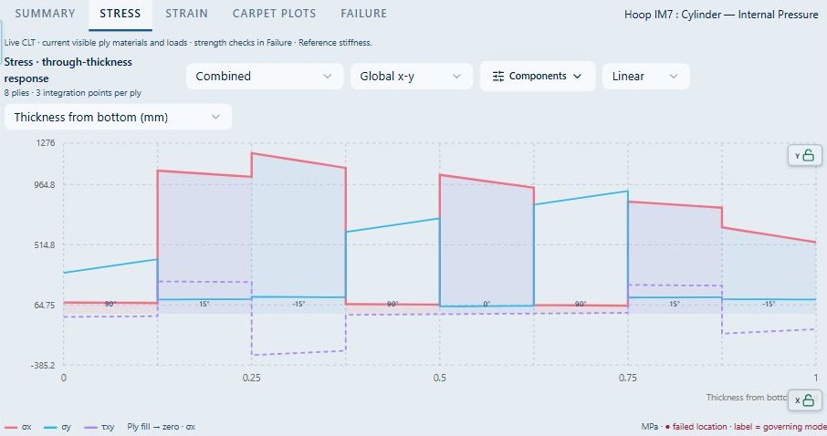
Step-by-step instructions · 4 steps

1. Choose response source, global or local axes, components and scale. See screenshot
2. Select thickness from bottom or the available alternate depth coordinate. Inspect ply interfaces and angle labels. See screenshot
3. Increase recovery nodes per ply in Settings when more sampling is useful, then check that the result source is still appropriate.
4. Use the resizable output region and axis locks to inspect the complete plot. See screenshot

09

Build and interpret a failure envelope

An envelope traces first-failure capacity in a selected pair of load components. Each ray is evaluated with the selected material criterion and laminate response; the displayed curve joins sampled directions.

Step-by-step instructions · 4 steps

1. Choose the envelope axes, supported theories and the fixed/background load state in Failure inputs.
2. Generate or update the envelope; inspect the completion/evaluation status and units.
3. Right-click the envelope plot to show markers when you need to see the calculated samples.
4. Compare criteria only when each has valid material data. A curve farther from the origin is not proof that its theory is more accurate.

10

Follow progressive failure

Progressive analysis ramps the selected loads, evaluates ply criteria and updates damage/stiffness according to the chosen method. First-ply failure and last-ply/terminal response answer different questions.

Step-by-step instructions · 4 steps

1. Set criterion, ramp, step count, search limit and stopping rule in the Failure inputs.
2. Choose whether saved thermal/cure effects, cure shrinkage and moisture expansion are reused; rerun the relevant solver after changing those inputs.
3. Read first activations, damaged plies, load factor and retained stiffness together.
4. Use the selected event, ply and pseudo-time controls to inspect the corresponding response. Pseudo-time in the proportional ramp is the load multiplier, not seconds.

11

Explore elastic design space with 2D and 3D carpet plots

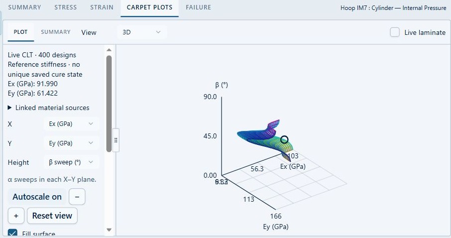
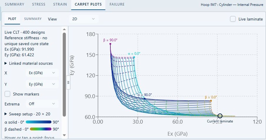
Carpet plots sweep two existing absolute-angle families while retaining ply materials, thicknesses, ordering and angle signs. Choose two different outputs such as Ex, Ey, Gxy, νxy, A11/A22 or D11/D22, then select a 2D carpet or 3D surface.

Step-by-step instructions · 4 steps

1. Choose distinct α and β families already present in the laminate and set increasing 0–90° bounds with 2–21 samples per sweep. See screenshot
2. In 3D, choose which sweep lies in the plane and which output is vertical. Filled surfaces default on at 55% opacity; switch fill, mesh, autoscale, extrema and other display aids independently. See screenshot
3. Drag the divider to give controls or plot more room. The 2D/3D selector stays at the top, and the live laminate remains beside the 3D plot. See screenshot
4. Hover a point to inspect the exact color-coded candidate. Display minima and maxima when locating the evaluated extrema, then verify balance, symmetry and manufacturability for that candidate. See screenshot

12

Optimize lamina and microstructure inputs

Lamina / Micro mode builds the same 2D and 3D study workflow around microstructure inputs rather than ply angles. It uses the selected micromechanics model, linked constituents, editable empirical parameters, and available thermal or moisture data.

Step-by-step instructions · 5 steps

1. Choose the micromechanics record and confirm its linked fiber, matrix, filler or void records. Missing required inputs stop the study instead of silently substituting a hidden constant.
2. Select two inputs from the variables relevant to that model: composition, aspect ratio, orientation, crimp, weave or braid terms, void knockdown, constituent-retention factors, or editable transport closures.
3. Choose elastic, strength, density, specific heat, conductivity, thermal diffusivity, moisture diffusivity or moisture saturation as the mapped output.
4. Set bounds, fixed slices and constraints. Use 2D contours or filled 3D surfaces with extrema and autoscale controls to examine maxima, minima and trade-offs.
5. Save the snapshot before applying a candidate. Applying writes the chosen active model parameters back to the micromechanics record; downstream laminate and structural results should then be rerun.

13

Run a bounded laminate optimization

Laminate mode searches discrete ply angles for a selected mechanical load case. Objectives are lowest feasible areal mass, greatest first-failure load factor, or greatest absolute selected mid-plane strain at first failure.

Step-by-step instructions · 6 steps

1. Choose Laminate in Optimize Inputs, then select the structural case, objective, first-ply criterion, allowed angles and required load factor.
2. For mass, set minimum/maximum ply counts. Strength and strain hold the current ply count fixed.
3. Choose symmetric construction, balanced pairs and minimum angle content as needed. Review the angle-content guidance.
4. Set a repeatable seed and evaluation budget in Search settings. The supported range is 1–64 plies and 20–2000 evaluations.
5. Click Optimize. Read evaluated/feasible counts, convergence, trade-off plot and Best Found together. Drag the panel dividers to inspect the plots.
6. Apply candidate updates the existing laminate after confirmation. Create new laminate creates a separate candidate-based record and leaves the original laminate and simulation link unchanged. Both actions remain disabled until a feasible candidate is available.

14

Save and compare optimization cases

Use Save snapshot in Inputs, beside the structural-case dropdown, after a result is available. Name the case so its objective and loading are recognizable.

Step-by-step instructions · 4 steps

1. Saving captures the inputs, load vector, search settings, candidates, convergence and best-found result; it also provides a CDS_DB download.
2. Open a saved case from Optimizations below Simulations. Saved inputs are read-only.
3. Select multiple cases for the comparison table and Ashby, bar or line views. Use axis properties and filters just as in Materials results.
4. Start New optimization for a fresh search. Changing current inputs does not rewrite an earlier snapshot.

15

Know what the search does not establish

Small spaces are exhaustively enumerated; larger spaces use seeded multi-start search. A budget limit or flat convergence curve is not proof of a global optimum.

Step-by-step instructions · 4 steps

1. Repeat large searches with different seeds and budgets.
2. Check contiguity, disorientation, manufacturing rules and damage tolerance separately.
3. Validate buckling, fatigue, joints, defects, delamination and environmental effects with suitable models and data.
4. Treat any claimed “best” design as best found within this defined search space and model.

16

Result, plot and export controls

Every result view keeps its own selectors, axes, cursor, scale, visibility and export actions. The active tab identifies the dataset being inspected; changing a display control does not recalculate the model.

Step-by-step instructions · 5 steps

1. Table, Ashby, Bar, Line, 2D and 3D select the presentation. Property, component, axis and contribution dropdowns select what is displayed.
2. Autoscale fits current data. Axis locks preserve chosen limits for comparison. Reset view restores the default camera or plot framing.
3. On 3D plots, Fill, opacity, mesh and extrema affect visibility only. Drag or use the documented keyboard controls to rotate, zoom and select designs.
4. Right-click a supported plot or table for image, CSV, XLSX, PDF or other available exports. CSV and XLSX preserve data; image and PDF preserve presentation.
5. Save Report opens report-content choices for the workflow image, written summary, connected-input tables and current key results. High-level and detailed modes change included evidence, not solver results.

17

Optimization control reference

Mode, objective, variable, constraint, bound, seed and budget controls define the search. Candidate, Apply, Create new, Save snapshot and comparison actions operate on the resulting study.

Step-by-step instructions · 4 steps

1. Mode selects Micro, Laminate or Process and determines the available variables and outputs.
2. Bounds restrict the search space. Constraints define feasibility. Seed makes a stochastic search repeatable; budget limits evaluations rather than proving convergence.
3. Optimize starts the search; Cancel stops it. Best Found is the best feasible candidate encountered in this configured study.
4. Apply candidate edits the linked record after confirmation. Create new preserves the original and creates a separate record. Save snapshot freezes the study inputs and results for comparison.

Chapter review

Retain the chosen candidate and evaluate it with the compatible study. Report the search bounds and evaluated constraints with the comparison.